Geospatial analysis has a long history in geography and cartography. Geospatial analysis aims to answer the question of where something happens and what impact that something has on neighboring areas.
Geospatial analysis requires spatial attribute values or geolocations for authors and their papers, extracted from affiliation data or spatial positions of nodes, generated from layout algorithms. Geospatial data can be continuous (i.e., each record has a specific position) or discrete (i.e., each set of keywords has a position or area-shape file – e.g., number of papers per country). Spatial aggregations (e.g., merging via ZIP codes, counties, states, countries, and continents) are common.
Cartographic generalization refers to the process of abstraction such as (1) graphic generalization: the simplification, enlargement, displacement, merging, or selection of entities without enhancing their symbology; and (2) conceptual symbolization: the merging, selection, and symbolization of entities, including enhancement – such as representing high-density areas with a new (city) symbol.
Geometric generalization aims to solve the conflict between the number of visualized features, the size of symbols, and the size of the display surface. Cartographers dealt with this conflict intuitively in part until researchers like Friedrich Töpfer attempted to solve them with quantifiable expressions.

4.7.1 Extract ZIP Code

Description

This algorithm parses the address information provided and extracts ZIP codes from it. Currently it accepts ZIP codes which are in United States of America format i.e. either XXXXX (short form) or XXXXX-XXXX (long form).

Pros & Cons

This algorithm facilitates quick Spatial analysis by extracting ZIP codes from a given address, which can be further processed. Its only limitation is that currently it only supports parsing of USA ZIP Codes or countries which have USA based ZIP Code format.

Implementation Details

The algorithm works as follows,

1. Get the address for each row & begin parsing for zip codes in the following manner,
   1. Save all groups of digits along with their start position, end position & length of the group of digits.
   2. Since the zip code, presumably, will be in the later portion of the address string, traverse the collected zip code candidates in the reverse fashion.
   3. If there is a 5 digit group then,
      1. Consider it as the primary zip code. If the user wants the ZIP code in truncated form then the algorithm will skip the checking for extension ZIP code.
      2. The extension of the ZIP code follows the primary zip code, so check if the previous group has length 4 and if so, then check if its distance from primary zip is less than or equal to 2. If yes, than consider this as the extension of the zip code.
      3. If there is no 4 digit group satisfying the above conditions then return null as the extension value.
      4. If there is no 5 digit group then return null for the primary zip code value. In this case, display a warning to the user that no ZIP code was found for this particular address string.

Usage Hints

The user has to provide 3 inputs; a file containing the addresses for which ZIP code parsing is required, whether to truncate the parsed ZIP code or not and name of the address column. If the plugin was unable to find any ZIP code then it will print a warning message and set the ZIP code to empty string. The data for ZIP codes can be in either short form i.e. XXXXX or long form i.e. XXXXX-XXXX. It will also accept ZIP code information in the following format,

XXXXX<Any Character(s) of Max Length = 2>XXXX.
The output of this algorithm will be the original input table with 1 column added containing the parsed ZIP code.

4.7.2 Generic Geocoder

Description

This algorithm provides a general-purpose geocoding functionality that is expanded on by other more specific geocoding algorithms (see Bing Geocoder). It supports four types of geocoding: address, country, U.S. states and U.S. ZIP codes.

Pros & Cons

1. Increase of code re-used with abstract classes that defines the common behaviors such as GUI layout, data handling, etc.
2. Standard GUI layout gives a professional look to the application. Once the user learns to use one geocoder, it will be the same for using other geocoder plugins.
3. Problems can arise if the inherited behaviors are not well defined, since a single change on the abstract class will cause changes on all sub-classes.

Applications

Plugins that use this interface provide geographical coordinate information for the geomap application. Scientists can then visualize their data geographically.

Implementation Details

This algorithm provides a common front-end behaviors algorithm for multiple geocoder plugins. It uses the MVC (Model-View-Controller) idea to facilitate the in-dependency and code reused implementation.

1. View
   - AbstractGeocoderFactory defined GUI layout, data validation and geocoder type selection. It contains a FamilyOfGeocoder member that refer to the related geocoder family (Generic, Bing, etc)
2. Controller
   - GeocoderAlgorithm processes the geolocation look up using the given Geocoder. The first look up is through invoking geocodingFullForm. If the look up failed, the second look up will be performed through invoking geocodingAbbreviation. It also provide error handling which analyzes the look up failures and provides appropriate warning message to user. In success, it generates a CSV output file with two additional columns that hold latitude and longitude values.
   - FamilyOfGeocoder contains four type of geocoders from the same family. There are address, country, U.S. states and U.S. ZIP codes.
3. Model
   - It uses the common geocoder model that is defined in edu.iu.sci2.model.geocode. It uses Geolocation that represents geographical coordinate and USZipCode that contains uzip (the first 5 digit ZIP code) and postbox number (the last 4 digits number in 9-digits ZIP code).
   - Each geocoder might holds its own model if needed

Usage Hints

The usage is provided on each geocoder wiki page. For example, Bing Geocoder.

Links

• Source Code
• External Package

Acknowledgments

The geocoding algorithm was authored, modified, integrated and documented by Chin Hua Kong. Many thanks to Chintan Tank first Generic Geocoder implementation that provide a based code to start from.

4.7.3 Bing Geocoder

Bing Maps account and API Key

In order to use the Bing Geocoder plugin, you need a Bing Maps account and an API Key. The following steps guide you through the process:

1. Go to https://www.bingmapsportal.com/

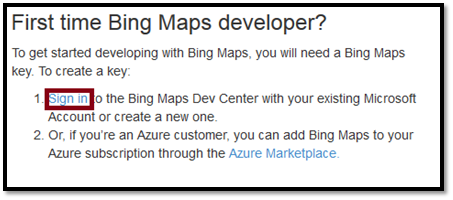
2. Under “First time Bing Maps developer?” click the sign in link (unless you are an Azure customer, then click the Azure Marketplace link).

3. You may be sent to a page that looks like this:

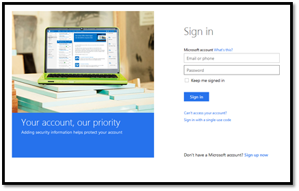
You will either need to sign in with an existing Microsoft account, or choose the bottom link that says “Sign up now” to create an account. If you have an account, simply sign in and skip to step six. If you do not, then click the “Sign up now” link and continue from here.

4. After clicking the “Sign up now” link you should see the following page:

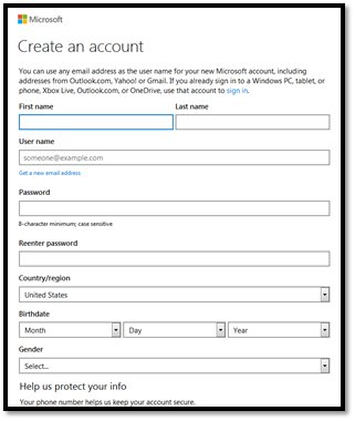
Fill this out and click “Create Account” when you are finished.

5. You will now need to verify the new account. Microsoft should have sent an email to the address you used to create your new account. Find this email and simply click on the blue bar that says “Verify    youremail@emailprovider.com” this should bring you to a page that looks like this:

Click “OK” and it should bring you back to the original page: https://www.bingmapsportal.com/

Then just follow the steps from step one. The only difference being that in step three you will sign in with your new account and skip to step six.

6. If you already have a Microsoft Account, then use this to sign in by clicking the Yes link. If you do not, then click on the Sign in with another account link.

7. Follow the instructions then click the “Create” button.

8. Now go to “My account” in the menu and choose “Create or view keys.”

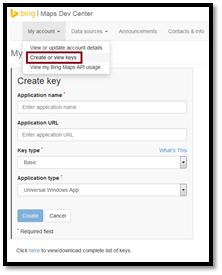
9. Fill out the “Create key” fields as shown below:

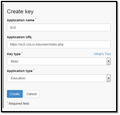
10. Click the “Create” button

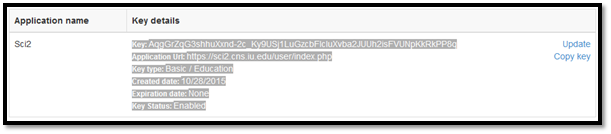
11. A box with the key should appear. Highlight everything in the box and hit Control-C ( you can try and click the “Copy key” link, but it does not work with all browsers). Then save the information in a Word document, .txt file, or in any format and location that you will be able to find and use easily. You will be asked for this key every time you use the Bing Geocoder in Sci2, so make sure it is easily accessible.

4.7.4 Congressional District Geocoder

Description

This algorithm converts the given 9-digits U.S. ZIP codes (ZIP+4 codes) into its congressional districts and geographical coordinates (latitude and longitude). The Benchmark is 50,000 ZIP codes per second. Download the plugin here.

Pros & Cons

1. 1. The algorithm is using a local database mapping with 25MB file size. It will increase the application size dramatically. So it is build as an external plugin
   2. For first execution in the same application window, the plugin required 5 seconds to load the database. The consequent execution will not required the pre-loading phase.
   3. Since some 5-digits ZIP codes contain multiple districts, the 9-digits ZIP codes is required for the conversion. Warning message will be printed to notice user if the given 5-digits ZIP codes contain multiple districts
   4. Congressional district might be varied by each election. The database would need to be maintained and updated relatively.

Applications

This plugin only support U.S. ZIP codes. It convert 9-digits ZIP codes to their belonging congressional district. It is an external plugin since the data size is so large. The dataset is based on the year 2008 election.

Implementation Details

Words for developers: Please do take a look at the ZIP code wiki at here to have a better understand on how U.S. ZIP+4 code system works. The first 5-digits number in ZIP code is called Uzip. The last 4-digits number in the ZIP+4 code is Post Office box number which can refer to here.

The challenge of the implementation is the design of the mapping model that used to look up congressional districts from ZIP+4 codes. To understand the metadata file (provided by GovTrack), create a mapping model with constant (O(1)) look up time and easy to managed. The implementation detail is documented in the source code.

The following will provide a high level view of the design.

1. 1. The algorithm is facilitated by the Model-View-Controller idea
   2. Model
      - The core of this implementation. Formed by ZipCodeToDistrictMap, PostBoxToDistrictMap and DistrictRegistry.
      - ZipCodeToDistrictMap hold a map of uzip to USDistrict and a map of uzip to PostBoxToDistrictMap.
      - PostBoxToDistrictMap hold a map of postBox to USDistrict and a map of wildcard to USDistrict map.
      - DistrictRegistry contains non-duplicated of USDistrict objects. It holds entire U.S congressional districts information.
      - USDistrict contains district label and geolocation. The class is imported from edu.iu.scipolicy.model.geocode package
   3. View - ZipToDistrictAlgorithmFactory contains all the view setup implementation, including title, windows and options
   4. Controller
      - ZipToDistrictAlgorithm prepares the model; parses the input ZIP codes to USZIPCode objects; performs the district look up, handles exceptions and saves the result to a CSV file.
      - The Look up is performed through ZipCodeToDistrictMap. If there isn't found a direct match of uzip to USDistrict, it will performed a look up through PostBoxToDistrictMap that holds by the uzip. Return USDitrict in success while throws ZipToDistrictException if no matched found
   5. Dependency: dist2geolocation.txt and zip4dist-prefix.txt

The output table contains all columns of the input table with three new columns (Congressional district, latitude and longitude).

Usage Hints

Here is a four steps guide to use the plugin:

1. 1. Load your input data file that contains 9-digits U.S. ZIP codes to be geocoded.
   2. Select Analysis > Geospatial > Congressional District Geocoder from menu bar. A window will be pop up
   3. Choose place name column that represents the ZIP code field in your data file.
   4. Press Ok button to start the geocoding

5-digits ZIP codes with multiple congressional districts, empty entries and invalid ZIP codes that failed to be geocoded will list in warning messages on the console.

The output of this algorithm is the original input table with additional 3 columns (Congressional district column, latitude column and longitude column). ZIP codes that failed to be geocoded will have blank entries.

Our benchmark is 50,000 ZIP codes per second.

Geomap the congressional districts

1. 1. Firstly, you might want to aggregate your data based on congressional district. To do this, you can follow user hints at here.
   2. You are ready to plot your aggregated result to geomap. It is recommended to plot the congressional district results on a country map due to some U.S. districts are located outside of the America Continents. To geomap the congressional districts, please follow the user hints at here.

Enjoy!!!

Links

• • Source Code
  • External Package
  • Home Page
  • GovTrack
  • WATCHDOG.NET
  • ZIP code's wiki

Acknowledgments

The geocoding algorithm was authored, implemented, integrated and documented by Chin Hua Kong. Many thanks to the Sprint team for providing advices and suggestions. Many thanks to GovTrack that provides ZIP to district mapping data and district's geolocation information. Thanks to Carl Malamud and Aaron Swartz, that make the data available on WATCHDOG.NET for GovTrack.

4.7.5 Geo Map (Circle Annotations) and Geo Map Colored Region Annotations

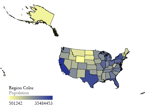
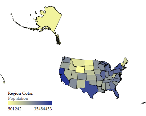
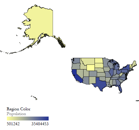
Choropleth Map

Color countries of the world or states of the US in proportion to numeric data.

Features

• • Optionally scale each individual dimension of numeric data logarithmically or exponentially.
  • Legends for each dimension show how all of the data corresponds to the visual representations.

Examples

Download source CSV
Download PDF

Usage Hints

• • It may be difficult to see any color coding applied to comparatively small regions on the map. In this case you may wish to geocode your region names as (longitude, latitude) coordinates and use the Proportional Symbol Map, perhaps disabling circle size coding and exterior color coding, then using interior color coding for whichever column you would have used with the Choropleth Map.

Usage Hints

• • Source Code

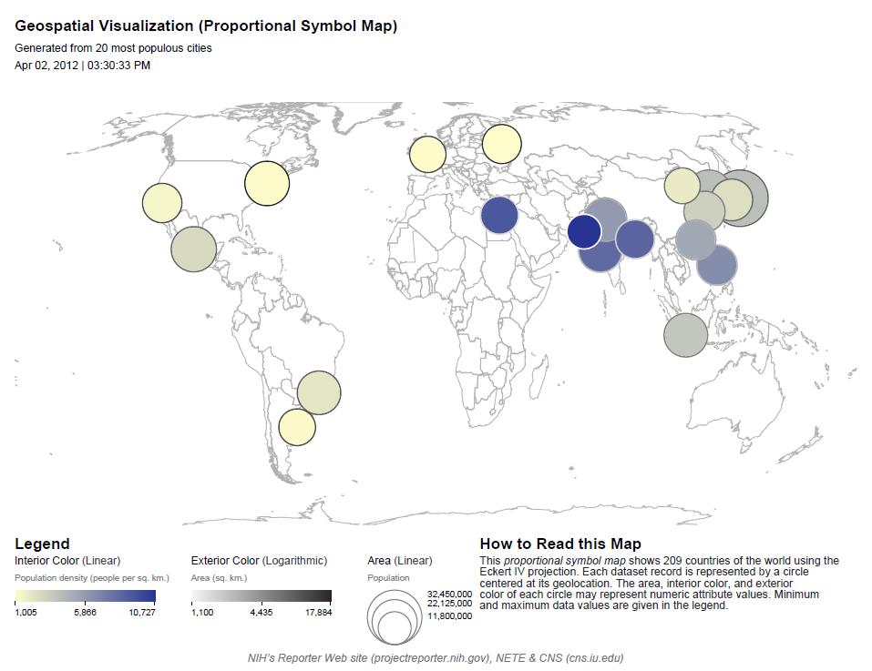
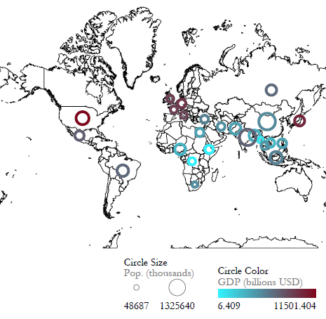
Proportional Symbol Map

Takes a table of geospatial coordinates associated with up to 3 numeric attributes and visualizes them as symbols overlaid on a world or United States base map. The sizes and colors of the symbols are proportional to the associated numeric data.

Features

• • Optionally scale each individual dimension of numeric data logarithmically or exponentially.
  • Legends for each visualization dimension show how all of the data are represented visually.

Examples

Download PDF

Implementation Details

Expects a table with numeric attributes that:

• • Describe that datum's longitude in degrees (from -180 to +180).
  • Describe that datum's latitude in degrees (from -90 to +90).
  • Determine the size of the circle at that coordinate.
  • Determine the color of the circle at that coordinate.

Usage Hints

• • If you have region names but not latitude and longitude data in your table, you can still easily produce a circle-annotated map using the Geocoder algorithm, which will find the coordinate data for each region name and add it to the table.
  • There is no perfect map projection – the choice depends on your application. We recommend:
    • Albers equal-area conic if preserving area is important.
    • Lambert conformal conic if preserving angles (or shapes) is important.
    • Mercator if presenting a familiar and fairly standardized projection is important.
  • The color-region Geomap is not suitable if your data contains small countries. For example, Singapore is too small a geographic region to be visible on the map when the region is colored. We recommend the user select the circle Geomap if data on smaller geographic regions is important for analysis.
  • The color-region Geomap requires that each country be identified using its name from the list Country names recognized by Geo Maps.
  • The color-region Geomap requires that each U.S. state be identified using its name from the list U.S. state names recognized by Geo Maps.

Links

• • Source Code

4.7.6 Using Gephi to Render Networks Overlaid on Geo Maps

Loading and Saving Geovisualization Files in Sci2

This algorithm allows for the geospatial visualization of network data. The algorithm produces a network file and corresponding blank map. Gephi is used to edit the network produced by Sci2. Once the network has been edited in Gephi it can be exported in a format that will allow it to be overlaid on the map, facilitating visualization of the geospatial data. The following is a brief workflow explaining the process, beginning to end. For this visualization the LaszloBarabasi-collaborations.net file will be used. This network maps Albert-László Barabási and his collaborators.

1. Load the LaszloBarabasi-collaborations.net network in Sci2.

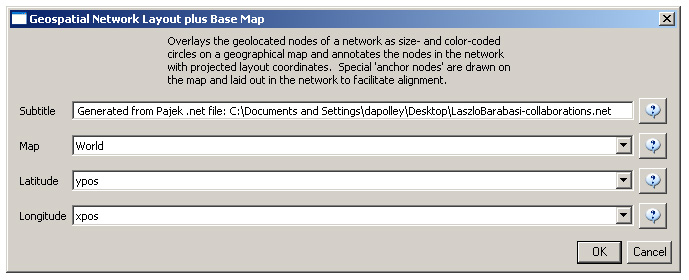
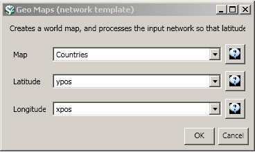
2. Once the network had been loaded in Sci2 run 'Visualization > Geospatial > Geospatial Network Layout with Base Map'. Make sure to set the lattitude to ypos and the longitude to xpos. By default, Sci2 tries to set the lattitude to xpos and the longitude to ypos and this will result in an inverted network that will not line up with the base map.

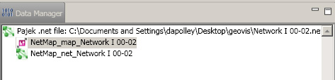
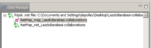
3. One this algorithm has been run the result will be two files in the data manager. A network (Laid out network) and a blank world map (base map with anchor points):

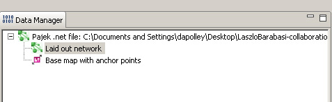
You will want to save both files. First, right click on the map file (bottom one) and save the file as a "PostScript" and select desired location. Before you open the map in an image editing software program you will likely need to convert from the PostScript file to a PDF. If you have the Adobe Creative Suite, you can do this by simply double-clicking on the PostScript file. If you do not have Adobe Creative Suite you can use this site to convert between the two file types http://www.ps2pdf.com/.  Now, right-click on the network file (top one) and save the file as GraphML (Prefuse) and select the desired location. Note, you may still need to change the network file type to a .graphml file.

Once the network file has been saved as a .graphml it can be loaded into Gephi. (If you do not currently have Gephi, it is freely available here and Gephi tutorials have been made available here.)

Manipulating the Network File in Gephi

1. When you open Gephi select "Open graph file..." under the New project heading in the popup window. If you inadvertently closed the popup window, then simply go to "File" and select "Open." Find the folder where you saved the network file and load the .graphml version of the network file. The "Import Report" pop-up will display, informing you that the network will be loaded as an undirected network. Click OK.

2. Once the network has been loaded you can view the graph in the "Overview" panel. The network had two nodes that correspond to two dots on the map file. These nodes will help you when you overlay the network on the map. In order to make these nodes more visible in the network file you may want to change their color.

3. Go to the "Data Laboratory" tab in the top left-hand corner of the Gephi tool.

4. Make sure you have the "Nodes" tab selected, you will see a list of all the nodes in the network. By scrolling down to the bottom of the node list you will notice that two nodes are labeled "Near Alaska" and "Near Antarctica" and are both anchor nodes (look at the isAnchor column).

5. Right click on the first anchor node and select the "Edit node" option. This will bring up the Edit function on the left-hand side of the screen:

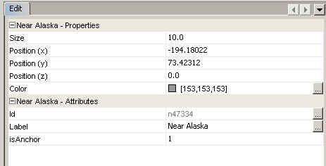
6. You can now adjust the color to make the nodes more visible. Repeat the same process for the node near Antarctica.

7. Return to the "Overview" tab and you will notice that the nodes have been colored based on your specifications.

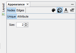
8. Next you will want to resize the nodes and decrease the edge weight to make the network more visible in the resulting visualization. You can change the size by going to "Window" and selecting "Appearance." A workspace window should appear to the left of the "Graph" screen labeled "Appearance." Make sure the "Nodes" tab is selected and the "Unique" tab under that. Then select the icon that looks like three circles, each a little bigger than the other, this is the sizing tool. Then adjust the node size to 2 as shown here:

9. Decrease the Edge weight using the slider bar at the bottom of the 'Graph' screen:

Saving the Network in Gephi

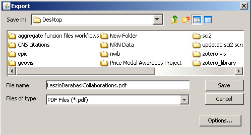
1. There are several ways to overlay the network file on the map file. It can be done entirely in Photoshop or it can be done by using a combination of Adobe Illustrator and Photoshop. The easiest way is to first export the network file you have edited with Gephi to a PDF format.

Creating the Visualization in Photoshop

1. Open the map file (blank map generated in Sci2)  in photoshop. You may need to rotate the image. This can be done by selecting the layer and clicking 'Edit > Transform > Rotate'.

2. Next, open the PDF saved from Gephi in Adobe Illustrator. You can delete the path that borders the entire image and use the select arrow to select the entire network. Then click 'Edit > Copy'.

3. Now, in the map file select 'Edit > Paste''. You will want to select paste as pixels. This will create a new layer in the map Photoshop file. The network will appear as a new layer on top of the map.

4. Any resizing that needs to be done in order to line up the colored nodes on the network file and their corresponding dots on the map file can be done by selecting the network image layer and using 'Edit > Transform > Scale'. Tip: hold down shift while doing the transform and it will be done to scale.

5. You can remove the colored nodes that are used to line up the images by using the eraser tool.

6. When you are finished editing the image you will want to merge both layers prior to saving the file. You can select both layers in the layers window to the right by using Ctrl click. Then right click and select "Merge Layers".

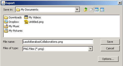
7.  In order to save the visualization once it has been created in Photoshop go to 'File > Save As' and then select an appropriate file name and file format, such as JPEG.

The resulting image will look like this:

Creating the Visualization in Gimp

Gimp offers an open source alternative to costly software like Adobe Photoshop. Gimp works really well for the purpose of overlaying network images generated by Sci2 and Gephi on geomaps. For more information or to download the tool see the Gimp website.

.

Here is the process for overlaying the network on the geomap created from the LaszloBarabasi-collaborations.net:

1. Open the map PDF file exported from Sci2 in one Gimp file.

2. Open the network PDF file exported from Gephi in another Gimp file.

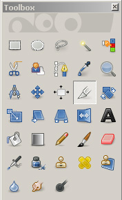
3. You will most likely need to crop the network image. You can either use 'Tools > Transform > Crop' or the crop shortcut in the Toolbox:

4. Once the image is cropped, copy the image, 'Edit > Copy'.

5. Paste the image as a new layer in the map file, 'Edit > Paste as > New Layer'.

6. The new layer (network overlay) will need to be made transparent, 'Layer > Transparency > Color to Alpha...'. This will make the geomap layer visible under the network overlay.

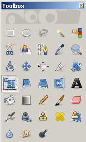
7 The network overlay will need to be scaled, allowing for the anchor nodes to line up with their corresponding positions on the map (near Alaska and near Antarctica. The easiest way is select the Scale tool from the Toolbox:

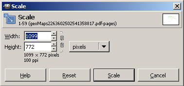
Click on the network overlay layer and the scale tool pop-up will appear. The layer to be scaled will appear with rectangles at each corner which allow users to re-size the layer with the mouse by clicking and dragging. Line up the anchor nodes on the network image with the corresponding points on the map image. Once the desired scaling has been achieved click the "Scale" button on the scaling pop-up:

8. Next you will need to merge the layers, 'Layer > Merge Down'.

9. Before the image can be saved it will need to be flattened, 'Image > Flatten Image'. 

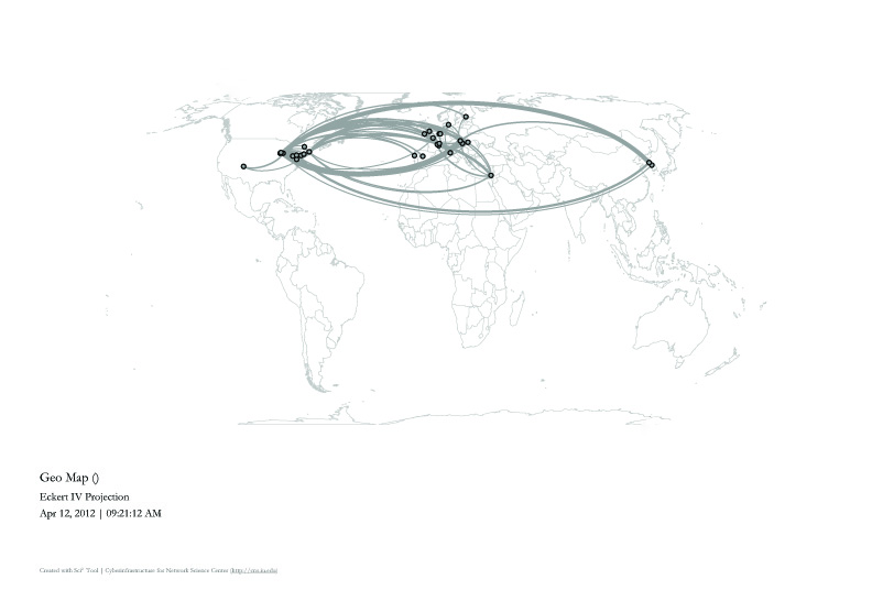
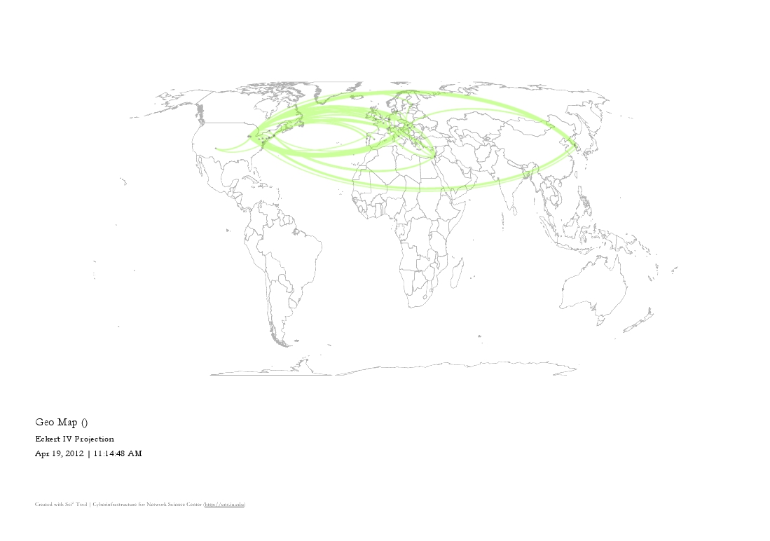
10. Save the visualization in desired format (recommended file format is .jpg). Below is an example of the LaszloBarabasi-collaborations.net file overlaid on a geomap. Note, the edges were colored in Gephi to make them more visible in the resulting visualization: