The topic or semantic coverage of a unit of science can be derived from the text associated with it. Topical aggregations (e.g., over journal volumes, scientific disciplines, or institutions) are common.
Topical analysis extracts the set of unique words or word profiles and their frequency from a text corpus. Stop words, such as 'the' and 'of' are removed. Stemming can be applied. Co-word analysis identifies the number of times two words are used in the title, keyword set, abstract and/or full text of a paper. The space of co-occurring words can be mapped providing a unique view of the topic coverage of a dataset. Similarly, units of science can be grouped according to the number of words they have in common.
Salton's term frequency inverse document frequency (TFIDF) is a statistical measure used to evaluate the importance of a word in a corpus. The importance increases proportionally to the number of times a word appears in the paper but is offset by the frequency of the word in the corpus.
Dimensionality reduction techniques are commonly used to project high-dimensional information spaces (i.e., the matrix of all unique papers multiplied by their unique terms, in a low, typically two-dimensional space).

4.8.1 Word Co-Occurrence Network

The topic similarity of basic and aggregate units of science can be calculated via an analysis of the co-occurrence of words in associated texts. Units that share more words in common are assumed to have higher topical overlap and are connected via linkages and/or placed in closer proximity. Word co-occurrence networks are weighted and undirected.

Mapping Topics and Topic Bursts in PNAS

This section documents how to create a co-word association map in order to study the structure and evolution of a research domain, in this case biology. It will highlight the process undertaken in the Ketan K. Mane and Katy Börner study (2004) that analyzes  a dataset comprising a complete set of 47,073 papers published in the Proceedings of the National Academy of Sciences (PNAS) from 1982-2001. The dataset was obtained from the Arthur M. Sackler Colloquium on Mapping Knowledge Domains. The colloquium was sponsored by the National Academy of Sciences and took place May 9-11, 2003 in the Beckman Center of the National Academy of Sciences, Irvine, CA. All attendees of the colloquium were provided access to the dataset. The raw data cannot be shared, but two derivative datasets will be used here to illustrate topic analysis. For more information see http://vw.indiana.edu/sackler03/#Database.

Co-Occurrence Map of the Topics and Topic Bursts in PNAS Publications

Using the smaller datasset of the top 50 keywords from the PNAS publications and the 4,699 a word co-occurrence network was created, resulting in a matrix. This word co-occurrence network has 50 nodes and 1082 edges that represent the relationships between the words. In order to enhance the visualization, the number of edges were reduced to the most meaningful relationships using the pathfinder network scaling algorithm (PFNet) (Mane & Börner, 2004). After running the PFNet algorithm the resulting word co-occurrence network was reduced to 50 nodes and 62 edges. You can visualize the network by following the steps below. You will need to have Pajek installed on your machine. If you do not have Pajek you can download the program for free by visiting the following site: http://mrvar.fdv.uni-lj.si/pajek/

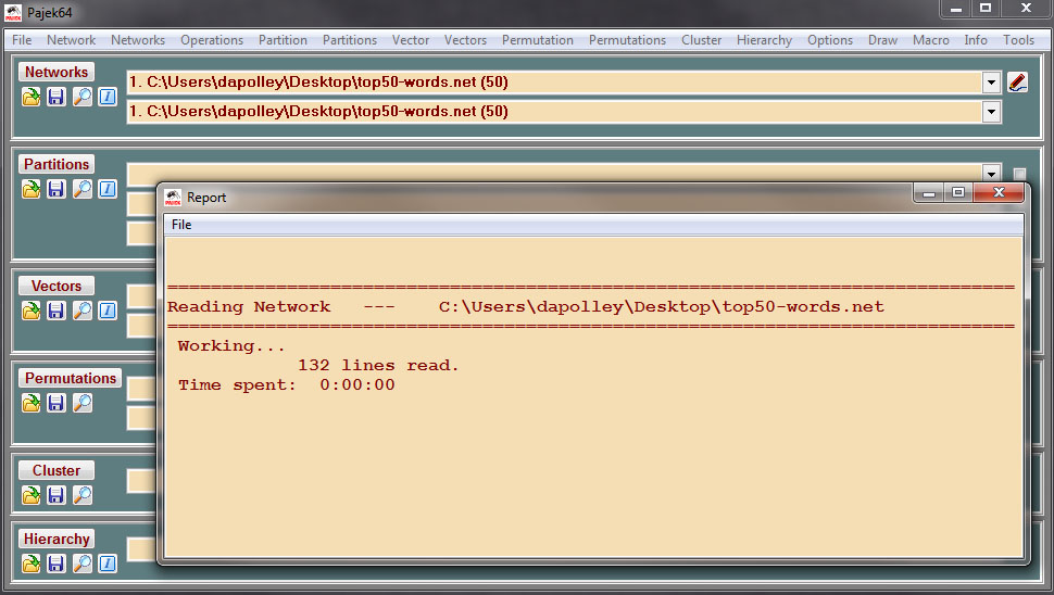
Download the PNAS_top50-words.net network file and load the file in Pajek by clicking on the open folder icon and navigating to where you have the network saved or by simply dragging and dropping the file into the "Networks" portion of the Pajek interface:

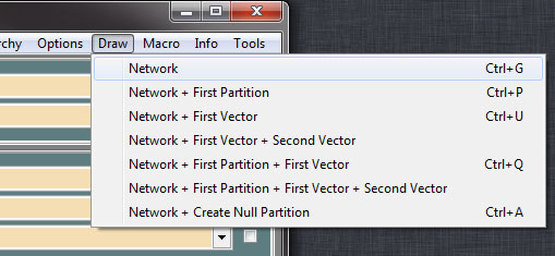
From there you simply need to select 'Draw > Network' from the menu at the top of the tool:

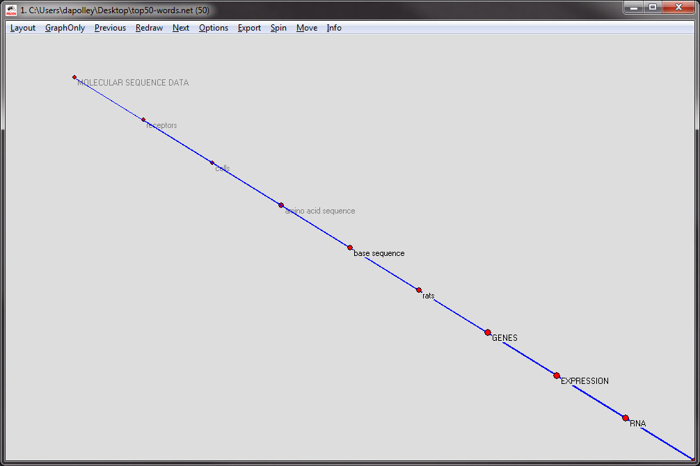
The graph should render in a separate window without any formatting:

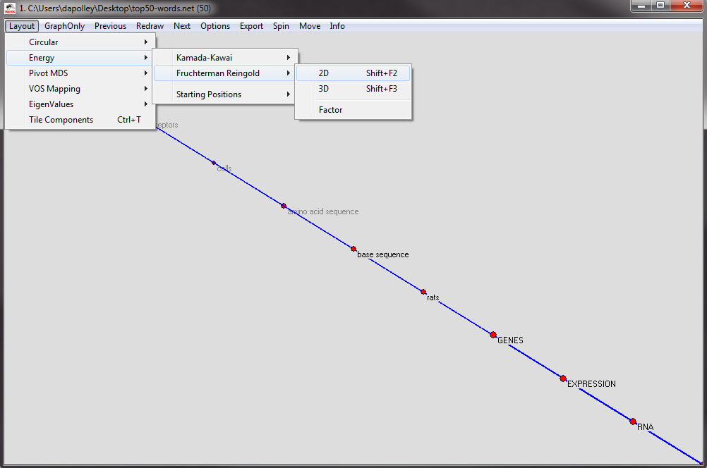
The first step is to change the layout. The layout used in Mane & Börner (2004) was the Fruchterman-Reingold 2D layout, 'Layout > Energy > Fruchterman Reingold > 2D':

The resulting layout should look something similar to this:

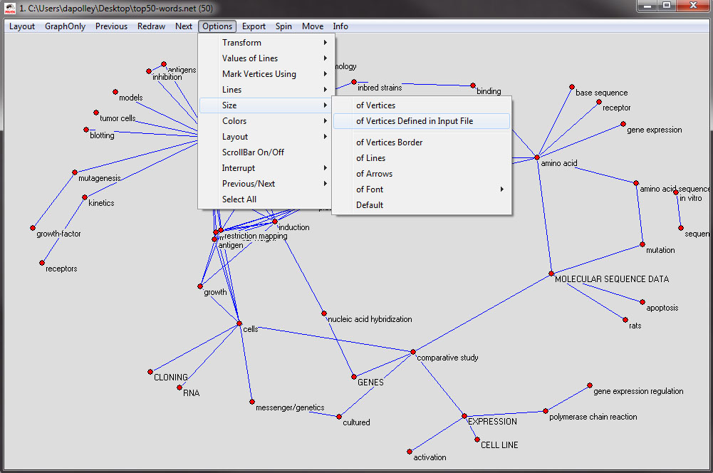
Next, you will want to resize the nodes, as specified in the original file, in  this case the nodes are sized based on the maximum burst level of the word represented by the node. From the menu at the top, select 'Options > Size > of Vertices Defined in the Input File':

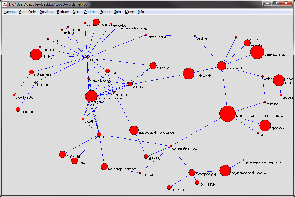
The resulting network should look roughly similar to this:

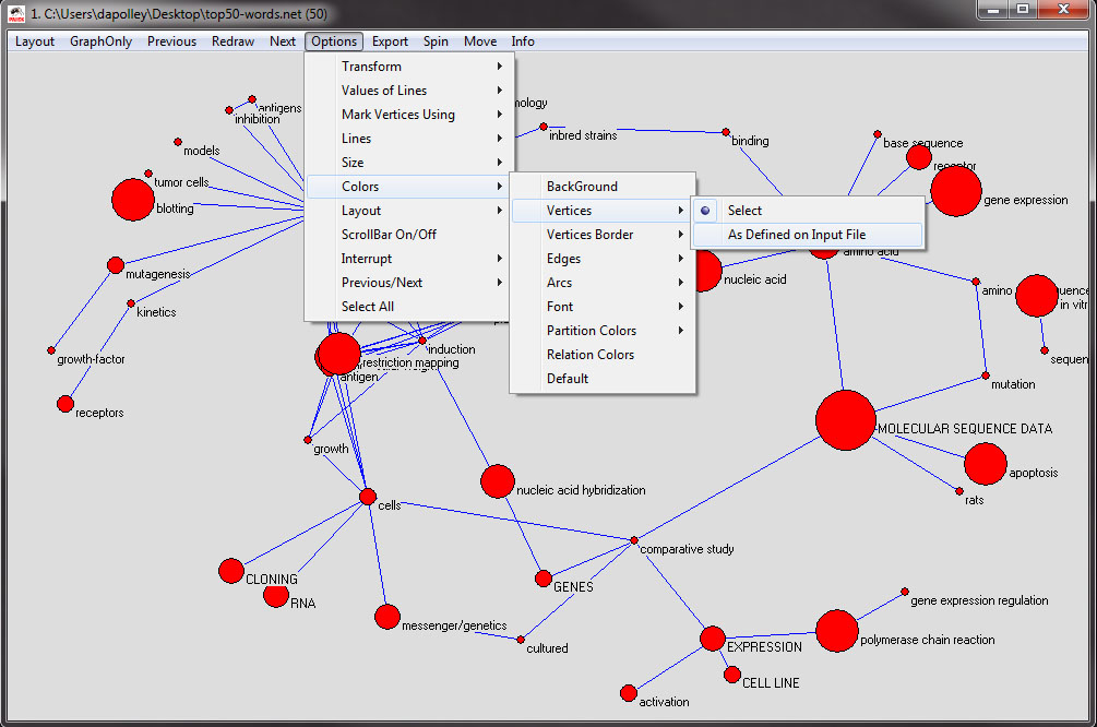
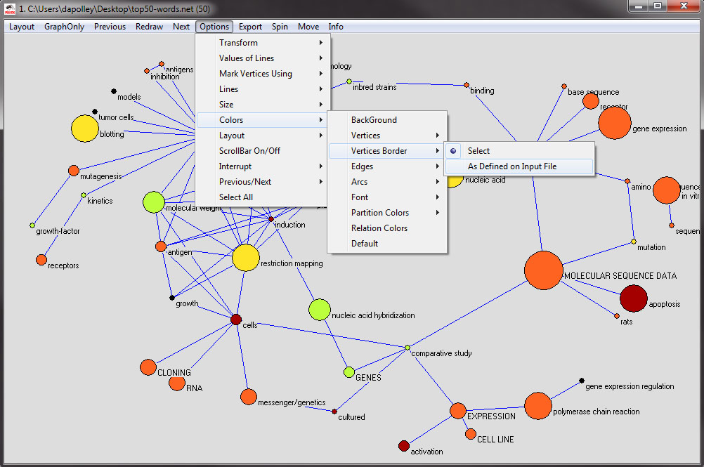
Next you will need to change the color of the nodes, which corresponds to the years in which the word was most often used. From the menu at the top of the tool, select 'Options > Colors > Vertices > As Defined on Input File':

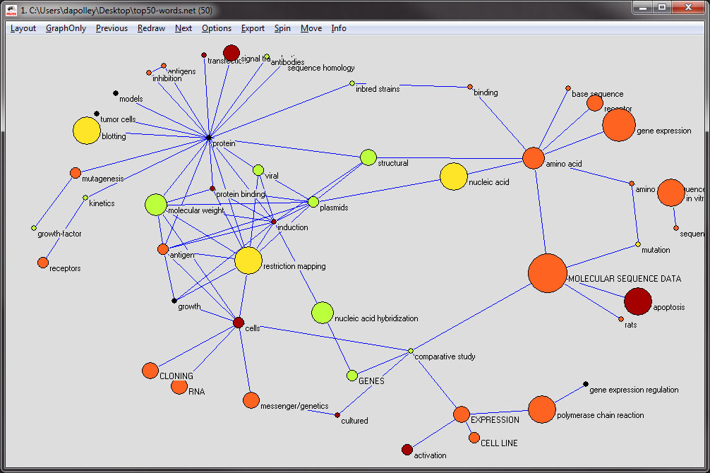
The resulting visualization should look something like the following. Also, at this point if you need to move around any of the nodes to eliminate overlapping, you can do so by clicking and dragging the nodes:

Next, you will want to change the node border color, which is colorized based on the the maximum frequency and the starting year of the first burst of the word represented by the node. From the menu at the top select, 'Options > Colors > Vertices Border > As Defined on Input File':

The resulting network will looks something like this:

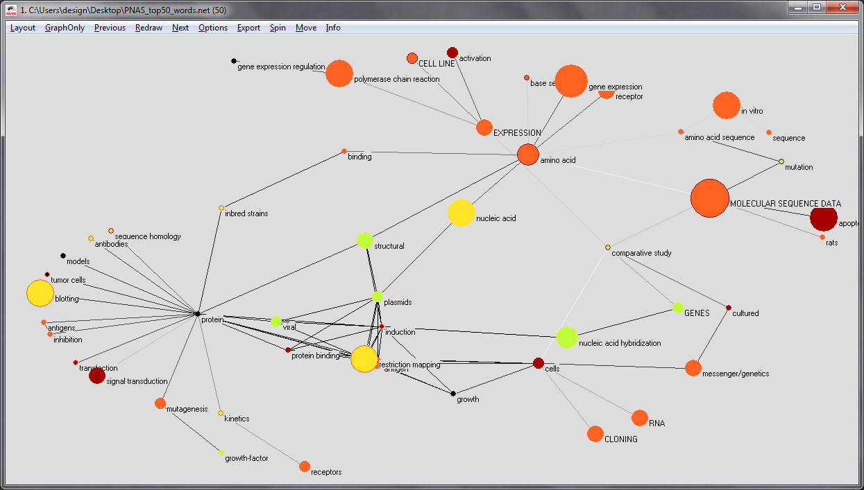
The next step is to set the color value of the edges to grey scale to make it easier to see the wight of the edges:

The resulting image should look something like this:

4.8.2 Map of Science via Journals

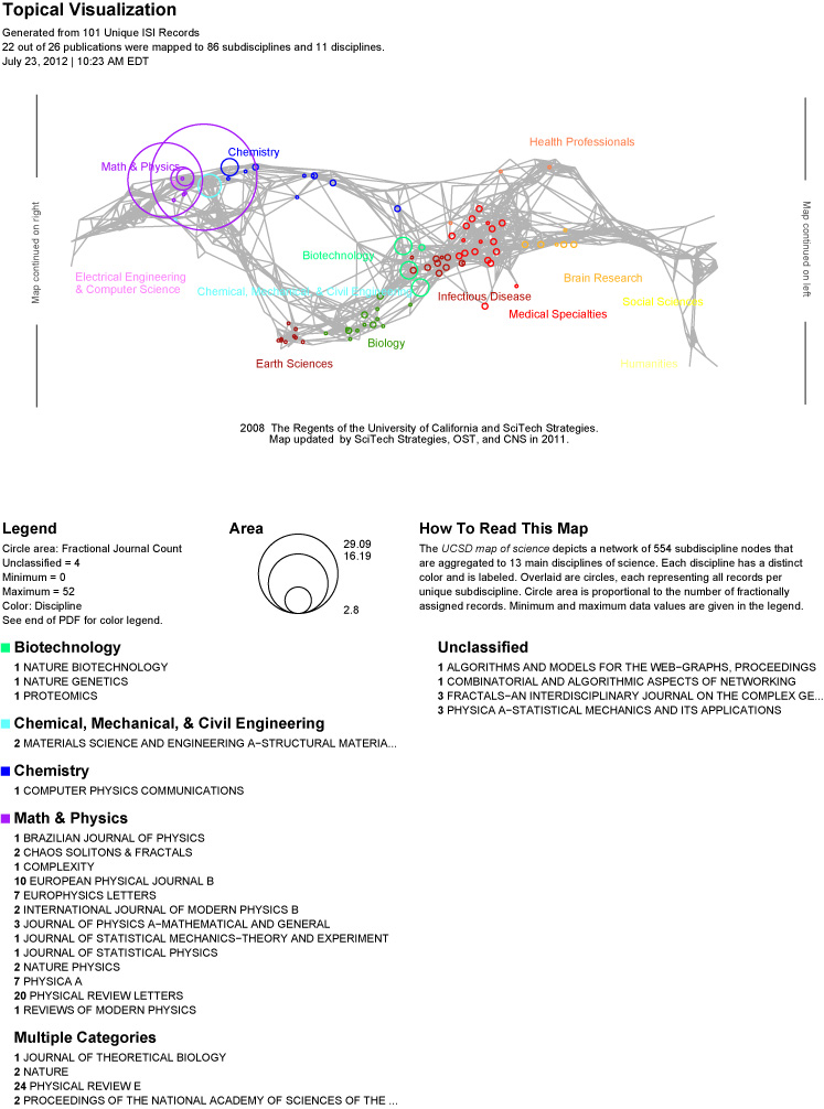
The Map of Science is a visual representation of 554 sub-disciplines within 13 disciplines of science and their relationships to one another, shown as points and lines connecting those points respectively. On top of this visualization is drawn the result of mapping a dataset's journals to the underlying sub-discipline(s) those journals contain. Mapped sub-disciplines are shown with size relative to the number matching journals and color from the discipline. For more information on maps of science, see http://mapofscience.com

There is a new plugin for the Map of Science visualization, make sure to download the plugin from 3.2 Additional Plugins

Input Parameters

Output

Below is an example of the Map of Science via Journals visualization with legend in the standard layout:

If you want to learn more about the Map of Science via Journals visualization the algorithm documentation.

4.8.3 Map of Science via 554 Fields

This visualization works exactly like Map of Science via Journals except instead of taking a collection of journal names as input and mapping them to the 554 fields it directly takes IDs of the 554 fields, which are integers from 1 to 554. Additionally, each field ID row can specify a non-integer integer value instead of listing the fields with multiplicity.