- 5.2.1 Funding Profiles of Three Universities (NSF Data)
- 5.2.2 Mapping CTSA Centers (NIH RePORTER Data)
- 5.2.3 Biomedical Funding Profile of NSF (NSF Data)
- 5.2.4 Mapping Scientometrics (ISI Data)
- 5.2.5 Burst Detection in Physics and Complex Networks (ISI Data)
- 5.2.6 Mapping the Field of RNAi Research (SDB Data)
5.2.1 Funding Profiles of Three Universities (NSF Data)
Cornell.nsf Indiana.nsf Michigan.nsf |
|
Time frame: | 2000-2009 |
Region(s): | Cornell University, Indiana University, Michigan University |
Topical Area(s): | Miscellaneous |
Analysis Type(s): | Co-PI Network |
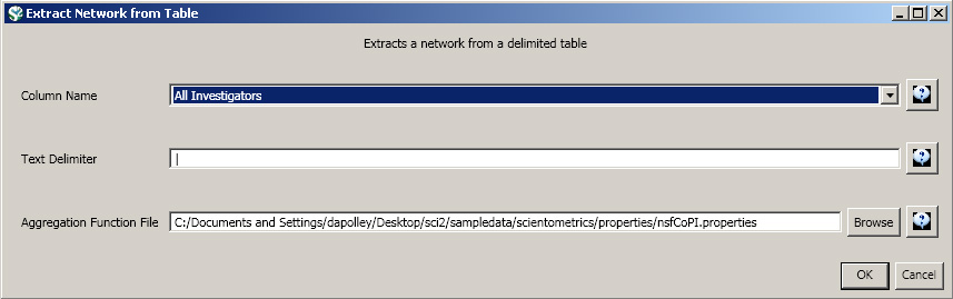
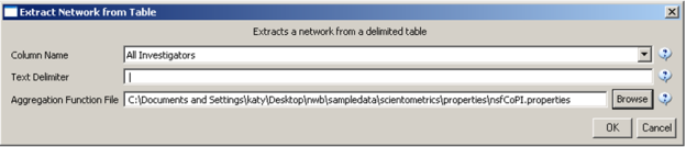
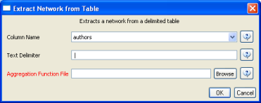
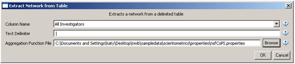
Load 'Cornell.nsf', 'Michigan.nsf', and 'Indiana.nsf' using 'File > Load" and following this path: 'yoursci2directory/sampledata/scientometrics/nsf' (if these files are not in the sample data directory they can be downloaded from 2.5 Sample Datasets). Use the following workflow for each of the three nsf files loaded. Select each of the datasets in the Data Manager window and run 'Data Preparation > Extract Co-Occurrence Network' using the following parameters (Note that the Aggregation Function File is 'yoursci2directory/sampledata/scientometrics/properties/nsfCoPI.properties'):
Aggregate Function File
Make sure to use the aggregate function file indicated in the image below. Aggregate function files can be found in sci2/sampledata/scientometrics/properties.
About NSF text delimiters:
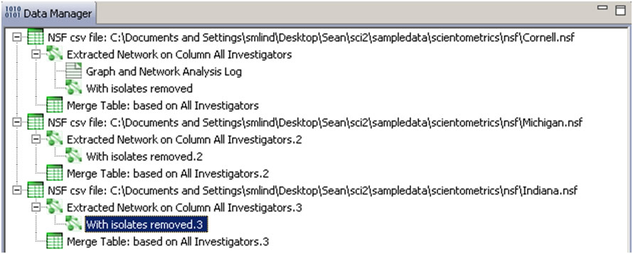
Two derived files per dataset will appear in the Data Manager window: the co-PI network and a merge table.
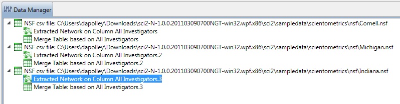
In the network, nodes represent investigators and edges denote their co-PI relationships. (To learn how the merge table can be used to further clean PI names, see section 5.1.4.2 Author Co-Occurrence (Bibliographic Coupling) Network.)
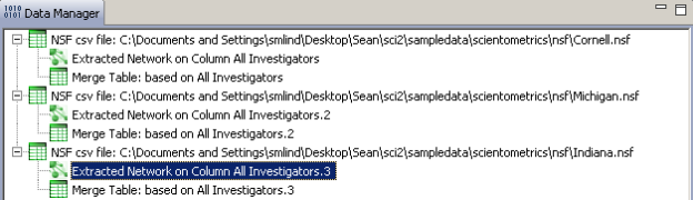
Choose the "Extracted Network on Column All Investigators" and run 'Analysis > Networks > Network Analysis Toolkit (NAT)' for each dataset. This will display the amount of nodes and edges, as well as the amount of isolate nodes that can be removed by running 'Preprocessing > Networks > Delete Isolates'.
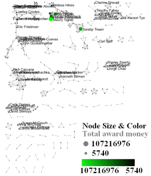
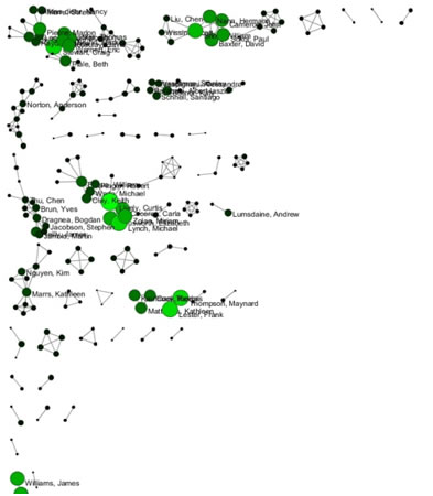
Select 'Visualization > Networks > GUESS' and run 'Layout > GEM' followed by 'Layout > Bin Pack' to visualize the network. Run the 'yoursci2directory/scripts/GUESS/co-PI-nw.py' script. Visualizations of the three university's co-PI networks are shown in Figure 5.23.
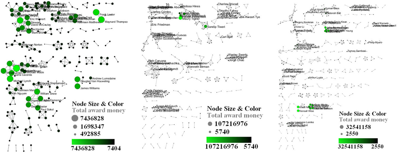
Figure 5.23: Co-PI network of Indiana University (top, left), Cornell University (top, right), University of Michigan (middle).
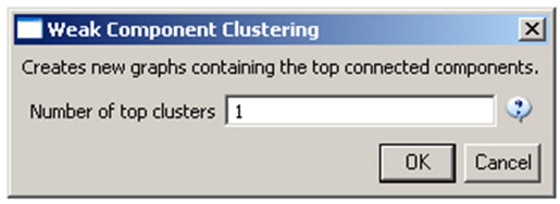
To see a more detailed view of any of the components in the network (e.g. the largest Indiana component) select the network with deleted isolates in the Data Manager:
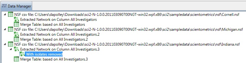
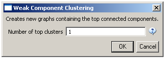
Then, run 'Analysis > Networks > Unweighted & Undirected > Weak Component Clustering' with the parameter:
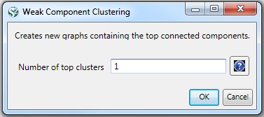
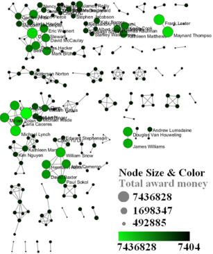
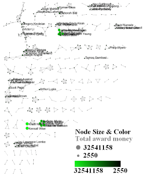
Indiana's largest component has 19 nodes, Cornell's has 67 nodes, and Michigan's has 55 nodes. Visualize Indiana's network in GUESS using the 'yoursci2directory/scripts/GUESS/co-PI-nw.py' script. Save the file as a jpg by selecting 'File > Export Image'. Use the "Browse..." option in the "Export Image – GUESS" popup window to select the folder in which you would like to save the image.
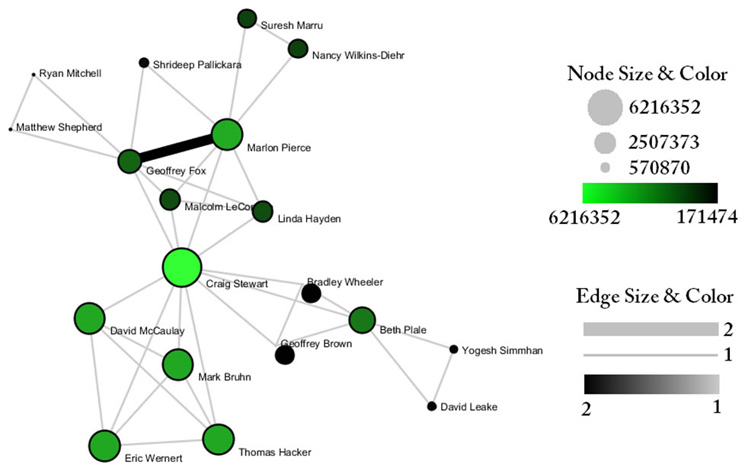
Figure 5.24: Largest component of Indiana University co-PI network. Node size and color display the total award amount.
To see the log file from this workflow save the 5.2.1 Funding Profiles of Three Universities (NSF Data) file.
5.2.1.1 Database Extractions
The database plugin is not currently available for the most recent version of Sci2 (v1.0 aplpha). However, the plugin that allows files to be loaded as databases is available for Sci2 v0.5.2 alpha or older. Please check the Sci2 news page (https://sci2.cns.iu.edu/user/news.php). We will update this page when a database plugin becomes available for the latest version of the tool.
The Sci2 Tool supports the creation of databases for NSF files. Database loading improves the speed and functionality of data preparation and preprocessing. To load the Indiana NSF file as a database, go to 'File > Load > and select yoursci2directory/sampledata/scientometrics/nsf/Indiana.nsf.' In the "Load" pop-up window, choose "NSF database." Cleaning should be performed before any other task using 'Data Preparation > Database > NSF > Merge Identical NSF People'.
To view a breakdown of each investigator from Indiana, run 'Data Preparation > Database > NSF > Extract Investigators'. View the table – notice that next to each investigator will be listed their total number of awards, total as the PI and as a Co-PI, the total amount awarded to date, as well as their earliest award start date and latest award expiration date.
To create Co-PI networks like those from the previous workflows, simply run 'Data Preparation > Databases > NSF > Extract Co-PI Network' on the cleaned database. Delete the isolates by running 'Preprocessing > Networks > Delete Isolates'.
As before, to visualize the network, select 'Visualization > Networks > GUESS' and run 'Layout > GEM' followed by 'Layout > Bin Pack'. Run the 'yoursci2directory/scripts/GUESS/co-PI-nw_database.py' script to apply the standard Co-PI network theme.

Figure 5.25: Indiana University Co-PI network using databases.
5.2.2 Mapping CTSA Centers (NIH RePORTER Data)
CTSA2005-2009.xls |
|
Time frame: | 2005-2009 |
Region(s): | Miscellaneous |
Topical Area(s): | Clinical and Translational Science |
Analysis Type(s): | PI-Institution Network, Co-Authorship Network |
Data doesn't always come in easily parsible formats. This study, a search for all recent grants to CTSA centers, requires some advanced searching and data manipulation to prepare the required data. The data comes from the union of NIH RePORTER downloads (see section 4.2.2.2 NIH RePORTER) and NIH ExPORTER data dumps (http://projectreporter.nih.gov/exporter/). Each CTSA Center grant was found and matched with its associated publications using a project-specific ID.
The resulting file, which contains all NIH Clinical and Translational Science Awards and their corresponding details from 2005-2009, is saved in an Excel file in 'yoursci2directory/sampledata/scientometrics/nih/CTSA2005-2009' (if the file is not in the sample data directory it can be downloaded from 2.5 Sample Datasets). The file contains two spreadsheets, one with publications and one with grants. Save each spreadsheet out as grants.csv and publications.csv.
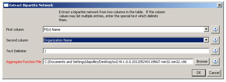
First load grants.csv in the Sci2 Tool using 'File > Load' and 'Standard csv format' in the "Load" pop-up. To view a bimodal network visualizing which main PIs associate with which institution, run 'Data Preparation > Extract Bipartite Network ' with the following parameters:
The resulting network can be visualized in GUESS and laid out using GEM, see Figure 5.26
. 
The network can also be visualized with the Bipartite-specific visualization. Run 'Visualization > Networks > Bipartite Network Graph' with the following parameters:
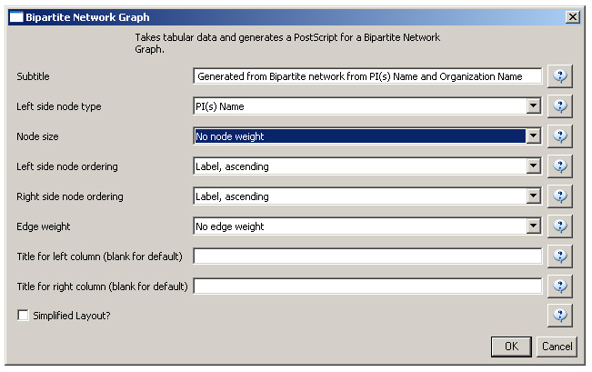
Sci2 will generate a visualization titled "Bipartite Network Graph PS" in the Data Manager. This network visualization can be saved as a PostScript file and the resulting visualization will look like this:
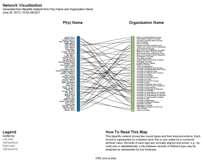
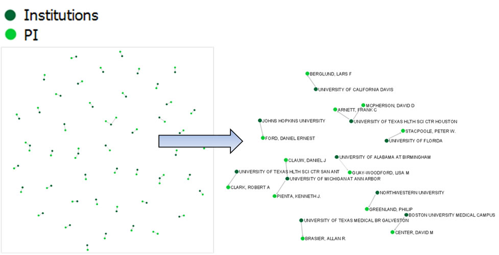
Figure 5.26: Bimodal institution-PI network for CTSA Centers.
Now load publications.csv as a standard csv and create a co-authorship network by running 'Data Preparation > Extract Co-Occurrence Network' with text delimiter set to " ; ". The parameter for Column Name should be set to "author." The resulting co-authorship network has 8,668 nodes, 26 isolates, and 50,129 edges (see Figures 5.27 and 5.28).

Figure 5.27: Co-authorship network of CTSA Center publications

Figure 5.28: Largest connected component of CTSA Center publication co-authorship network
To see the log file from this workflow save the 5.2.2 Mapping CTSA Centers (NIH RePORTER Data) log file.
5.2.3 Biomedical Funding Profile of NSF (NSF Data)
MedicalAndHealth.nsf |
|
Time frame: | 2003-2010 |
Region(s): | Miscellaneous |
Topical Area(s): | Biomedical |
Analysis Type(s): | NSF Organization-Program Network |
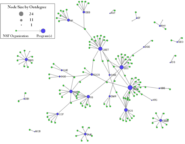
A NSF Organization-to-Program(s) bimodal network is exhibited here using data downloaded from the NSF Awards Search at (http://www.nsf.gov/awardsearch) on Nov 23th, 2009, using the query "medical AND health" in the title, abstract, and awards field, with "Active awards only" checked. This query yielded 286 awards (see section 4.2.2.1 NSF Award Search for data retrieval details).
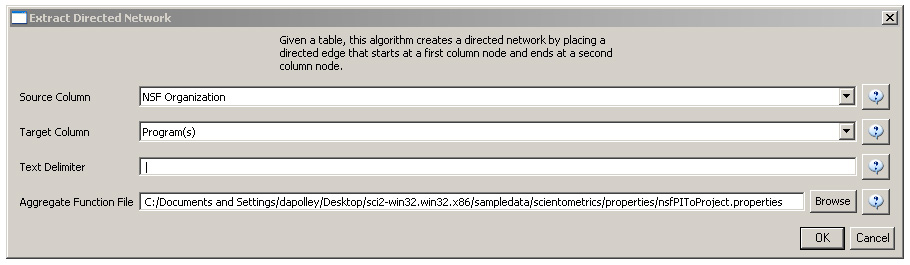
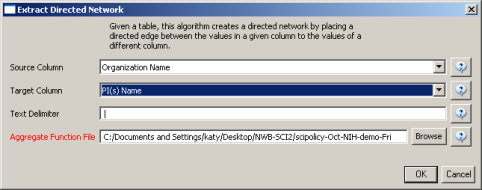
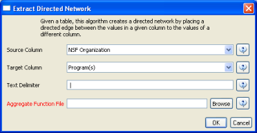
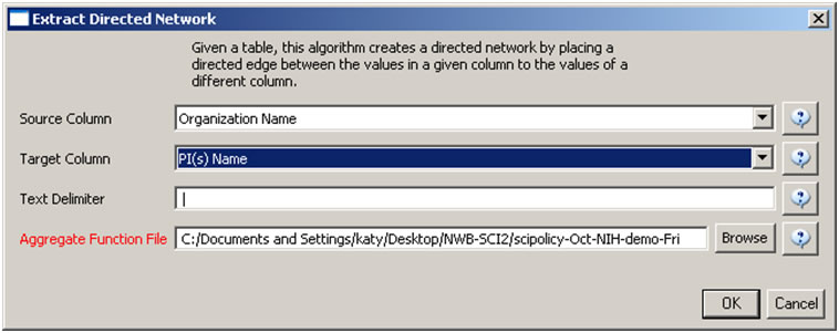
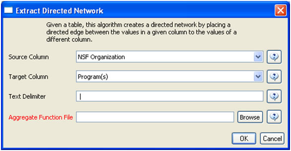
Load 'yoursci2directory/sampledata/scientometrics/nsf/MedicalAndHealth.nsf' in NSF csv format (if the file is not in the sample data directory it can be downloaded from 2.5 Sample Datasets). Then run 'Data Preparation > Extract Directed Network' with parameters:
Make sure to select the nsfPIToProject.properties for the aggregate function file.
About NSF Text Delimiters:
Select "Network with directed edges from NSF Organization to Program(s)" in the Data Manager and run 'Analysis > Networks > Unweighted and Directed > Node Indgree. Then select "Network with indegree attribute added to node list" in the Data Manager and run 'Analysis > Networks > Unweighted and Directed > Node Outdegree'. Select the resulting "Network with outdegree attribute added to node list" and run 'Visualization > Networks > GUESS' followed by ' Layout > GEM' and 'Layout > Bin Pack'.
In graph modifier interface:

![]()
Select "Colour" from the options directly below and choose desired color.
Then select "Show Label".
![]()
Select "Colour" and choose desired color.
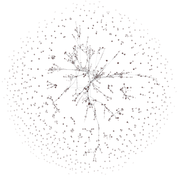
The resulting network is visualized in Figure 5.29.

Figure 5.29: Bimodal Network of NSF Organization to Program(s) of NSF Medical + Health Funding
To see the log file from this workflow save the 5.2.3 Biomedical Funding Profile of NSF (NSF Data) log file.
5.2.4 Mapping Scientometrics (ISI Data)
5.2.4.1 Document Co-Citation
Scientometrics.isi |
|
Time frame: | 1978-2008 |
Region(s): | Miscellaneous |
Topical Area(s): | Scientometrics |
Analysis Type(s): | Document Co-Citation Network |
Scientometrics is a discipline which uses statistical and computational techniques in order to understand the structure and dynamics of science. Here we use ISI data from the journal "Scientometrics" and Science of Science and Innovation Policy (SciSIP) data from NSF Awards Search.
Download Scientometrics.isi. Load the file using 'File > Load' and locating the downloaded file. This domain level dataset is ideal for document co-citation analysis, as the scale is large enough that the resulting network will paint a fairly accurate picture of document similarity within the domain of scientometrics.
New ISI File Format
Web of Science made a change to their output format in September, 2011. Older versions of Sci2 tool (older than v0.5.2 alpha) may refuse to load these new files, with an error like "Invalid ISI format file selected."
Sci2 solution
If you are using an older version of the Sci2 tool, you can download the WOS-plugins.zip file and unzip the JAR files into your sci2/plugins/ directory. Restart Sci2 to activate the fixes. You can now load the downloaded ISI files into the Sci2 without any additional step. If you are using the old Sci2 tool you will need to follow the guidelines below before you can load the new WOS format file into the tool.
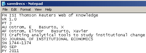
You can fix this problem for individual files by opening them in Notepad (or your favorite text editor). The file will start with the words:
Original file:
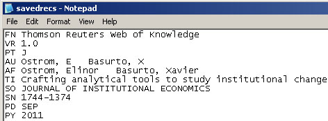
Just add the word ISI.
Updated file:

And then Save the file.
The ISI file should now load properly. More information on the ISI file format is available here (http://wiki.cns.iu.edu/display/CISHELL/ISI+%28*.isi%29).
Select the dataset "2126 Unique ISI Records" in the Data Manager window and run 'Data Preparation > Extract Paper Citation Network'.
Two files will appear in the Data Manager window: the paper-citation network and the paper information table.
Select the "Extracted paper-citation network" and run 'Preprocessing > Networks > Extract Nodes Above or Below Value' with the following parameters:
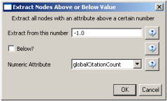
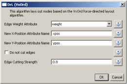
The produced network contains only the original ISI records. Select the resulting file and run 'Data Preparation > Extract Document Co-Citation Network'. Then, select the network and run 'Analysis > Networks > Network Analysis Toolkit (NAT)'. There are 2056 nodes, 26070 edges and 775 isolates in the network. Run 'Preprocessing > Networks > Delete Isolates' to remove all the isolates. Because this network is too dense to lay out in GUESS, run 'Visualization > DrL (VxOrd)' with the parameters:
Next, select "Laid out with DrL" in the Data Manager and run 'Visualization > Network > GUESS'. Run the following commands in the GUESS "Interpreter":
     >for n in g.nodes:
         if n.xpos is not None and n.ypos is not None:
             n.x = n.xpos * 10
             n.y = n.ypos * 10
     >resizeLinear(localcitationcount,1,50)
     >colorize(localcitationcount, gray, black)
     >resizeLinear(weight, .25, 8)
     >colorize(weight, "127,193,65,255", black)
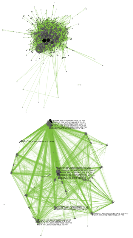
Go to "Graph Modifier" and choose 'Object: nodes based on -> > Property: localcitationcount > Operators: >= > Value: 20 > Show Label'. See Figure 5.21.

Figure 5.30: Document co-citation network for Scientometric.isi in GUESS without DrL edge cutting (top) and with DrL (VxOrd) (bottom).
To see the log file from this workflow save the 5.2.4.1 Document Co-Citation log file.
5.2.4.2 Geographic Visualization
Scientometrics.isi |
|
Time frame: | 1978-2008 |
Region(s): | Miscellaneous |
Topical Area(s): | Scientometrics |
Analysis Type(s): | Geospatial Analysis |
Using the dataset loaded from section 5.2.4.1, select '2126 Unique ISI Records' in the Data Manager. To find the latitude and longitudes of the locations of researches publishing in Scientometrics, run Analysis > Geospatial > Yahoo! Geocoder. Note that you will need a Yahoo Application ID in order to run this query. Enter your Yahoo Application ID (sign up for one here), "Address" for the Place Type, and the "Reprint Address" for the Place Column Name. Press 'OK'. This step may take several minutes to complete.

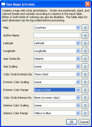
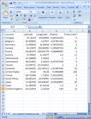
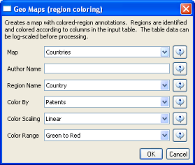
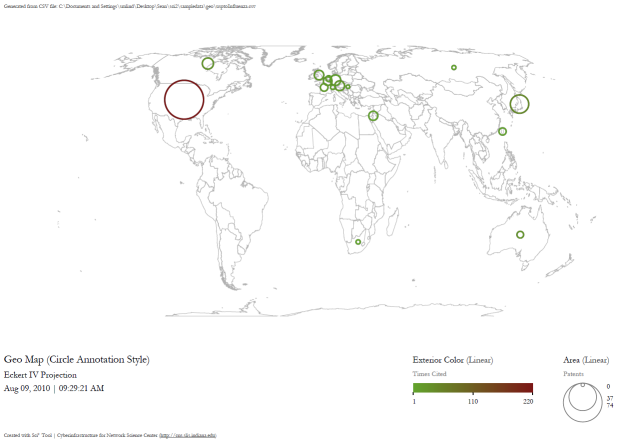
A new table will appear in the Data Manager labeled 'With Latitude & Longitude from 'Reprint Address'' containing all data from the initial table, plus columns with the Yahoo Geocoded Latitude and Longitude Coordinates. Select this file and run Visualization > Geospatial > Proportional Symbol Map using the parameters listed below.
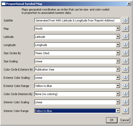
Save and view the resulting visualization using the directions described at 2.4 Saving Visualizations for Publication. This will be the result:
Figure 5.31: Scientometrics.isi geospatial visualization. Circle sizes represent times cited, colors represent publication year.
5.2.5 Burst Detection in Physics and Complex Networks (ISI Data)
AlessandroVespignani.isi |
|
Time frame: | 1990-2006 |
Region(s): | Indiana University, University of Rome, Yale University, Leiden University, International Center for Theoretical Physics, University of Paris-Sud |
Topical Area(s): | Informatics, Complex Network Science and System Research, Physics, Statistics, Epidemics |
Analysis Type(s): | Burst Detection |
5.2.5.1 Burst Detection
A scholarly dataset can be understood as a discrete time series: in other words, a sequence of events/ observations which are ordered in one dimension – time. Observations exist for regularly spaced intervals, e.g., each month or year.
The burst detection algorithm (see Section 4.6.1 Burst Detection) identifies sudden increases or "bursts" in the frequency-of-use of character strings over time. This algorithm identifies topics, terms, or concepts important to the events being studied that increased in usage, were more active for a period of time, and then faded away.
An analysis of publications authored or co-authored by Alessandro Vespignani from 1990 to 2006 will be used to illustrate the "burst" concept. Alessandro Vespignani is an Italian physicist and Professor of Informatics and Cognitive Science at Indiana University, Bloomington. In his publications, it is possible to see a change in research focus - from Physics to Complex Networks - beginning in 2001.
Load Alessandro Vespignani's ISI publication history using 'File > Load' and following this path: 'yoursci2directory/sampledata/scientometrics/isi/AlessandroVespignani.isi' (if the file is not in the sample data directory it can be downloaded from 2.5 Sample Datasets).
New ISI File Format
Web of Science made a change to their output format in September, 2011. Older versions of Sci2 tool (older than v0.5.2 alpha) may refuse to load these new files, with an error like "Invalid ISI format file selected."
Sci2 solution
If you are using an older version of the Sci2 tool, you can download the WOS-plugins.zip file and unzip the JAR files into your sci2/plugins/ directory. Restart Sci2 to activate the fixes. You can now load the downloaded ISI files into the Sci2 without any additional step. If you are using the old Sci2 tool you will need to follow the guidelines below before you can load the new WOS format file into the tool.
You can fix this problem for individual files by opening them in Notepad (or your favorite text editor). The file will start with the words:
Original file:

Just add the word ISI.
Original file:
And then Save the file.
The ISI file should now load properly. More information on the ISI file format is available here (http://wiki.cns.iu.edu/display/CISHELL/ISI+%28*.isi%29).
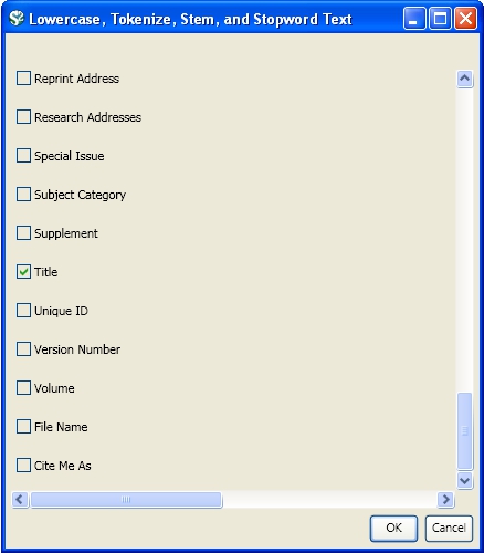
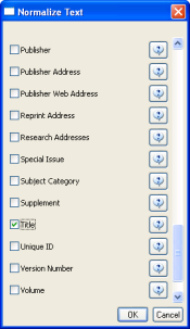
This analysis will detect the "bursty" terms used in the title of papers in the dataset. Since the burst detection algorithm is case-sensitive, it is necessary to normalize the field to be analyzed before running the algorithm. Select the table "101 Unique ISI Records" and run 'Preprocessing > Topical > Lowercase, Tokenize, Stem, and Stopword Text.' Check the "Title" box to indicate that you want to normalize this field:
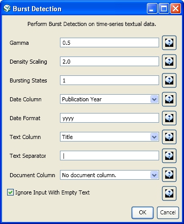
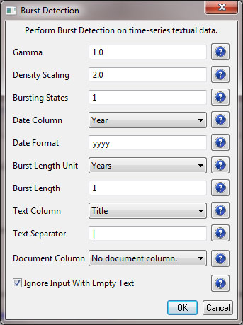
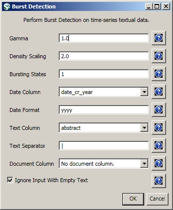
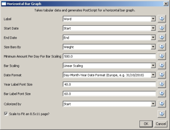
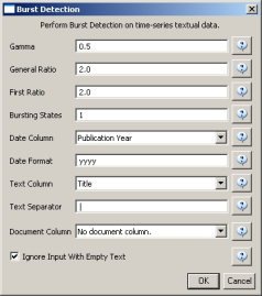
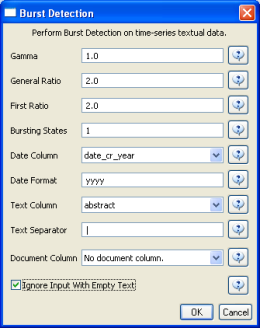
Select the resulting "with normalized Title" table in the Data Manager and run 'Analysis > Topical > Burst Detection' with the following parameters:
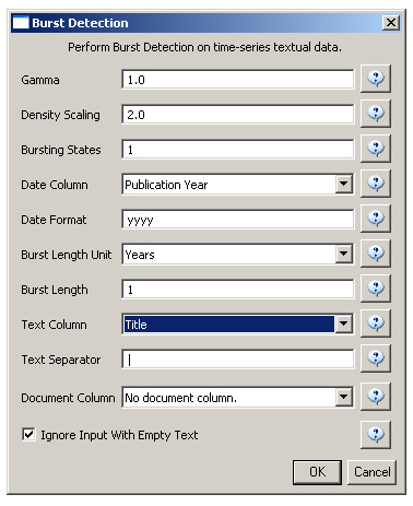
The "Gamma" parameter is the value that state transition costs are proportional to. This parameter is used to control how easy the automaton can change states. The higher the "Gamma" value, the smaller the list of bursts generated.
The "Density Scaling" parameter determines how much 'more bursty' each level is beyond the previous one. The higher the scaling value, the more active (bursty) the event happens in each level.
The "Bursting States" parameter determines how many bursting states there will be, beyond the non-bursting state. An i value of bursting states is equals to i + 1 automaton states.
The "Date Column" parameter is the name of the column with date/time when the events / topics happens.
The "Date Format" specifies how the date column will be interpreted as a date/time. See http://docs.oracle.com/javase/6/docs/api/java/text/SimpleDateFormat.html for details.
The "Text Column" parameter is the name of the column with values (delimiter and tokens) to be computed for bursting results.
The "Text Separator" parameters determines the separator that was used to delimit the tokens in the text column.
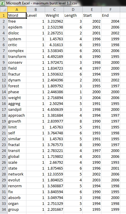
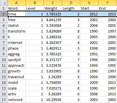
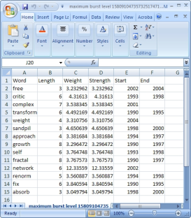
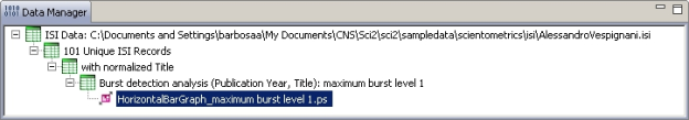
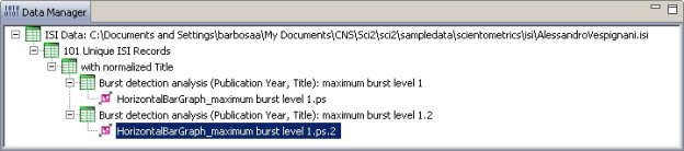
View the file "Burst detection analysis (Publication Year, Title): maximum burst level 1". On a PC running Windows, right click on this table and select view to see the data in Excel. On a Mac or a Linux system, right click and save the file, then open using the spreadsheet program of your choice.
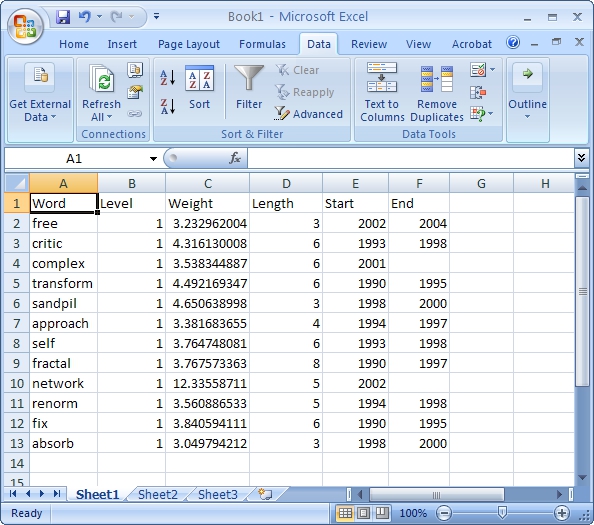
In this table, there are six columns: "Word," "Level," "Weight," "Length," "Start," and "End."
The "Word" field identifies the specific character string which was detected as a "burst." The "Length" field indicates how long the burst lasted (over the selected time parameter).
The "Level" is the burst level of this burst. The higher burst level, the more frequent the event / topic happens.
The "Weight" field is the weight of this burst between its "Length". A higher weight could be resulted by the longer "Length", the higher "Level" or both.
The "Length" is the period of the burst. It is generated based on (Start - End + 1).
The "Start" field identifies when the burst began (again, according to the specified time parameter).
And the "End" field indicates when the burst stopped. An empty value in the "End" field indicates that the burst lasted until the last date present in the dataset. Where the "End" field is empty, manually add the last year present in the dataset; in this case, 2006.

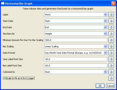
After you manually add this information, save this .csv file somewhere in your computer. Reload the .csv file into Sci2 using 'File > Load'. Select 'Standard csv format' int the pop-up window. A new table will appear in the Data Manager. To visualize the table that contains the results of the Burst Detection algorithm, select the table you just loaded in the Data Manager and run 'Visualization > Temporal > Temporal Bar Graph' with the following parameters:
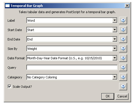
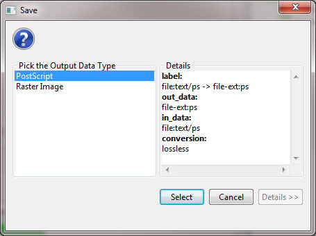
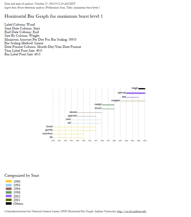
Temporal bar graphs are used to visualize numeric data over time, generating labeled horizontal bars. A PostScript file containing the horizontal bar graph will appear in the Data Manager.
Open and view the file using the workflow from Section 2.4 Saving Visualizations for Publication.

The resulting analysis indicates a change in the research focus of Alessandro Vespignani for publications beginning in 2001. For example, the bursting terms "fractal," "growth," "transform," and "fix" starting at 1990 are related to Vespignani's Ph.D., entitled "Fractal Growth and Self-Organized Criticality" in Physics. Other bursts also related to Physics follow these, such as "sandipil." After 2001, bursting terms like "complex," "network," "free," and "weight" appear, signifying a change in Vespignani's research area from Physics to Complex Networks, with a larger number of publications on topics like "weighted networks" and "scale-free networks."
Now, let's run the Burst Detection algorithm again for the same dataset but for a different value for the 'Gamma' parameter. Select the table 'with normalized Title' in the Data Manager and run 'Analysis > Topical > Burst Detection' with the following parameters:
Notice that the value for the gamma parameter is now set to 0.5. The parameter gamma controls the ease with which the automaton can change states. With a smaller gamma value, more bursts will be generated. Running the algorithm with these parameters will generate a new table named "Burst detection analysis (Publication Year, Title): maximum burst level 1.2" in the Data Manager.

Again where the "End" field is empty, manually add the last year present in the dataset; in this case, 2006.
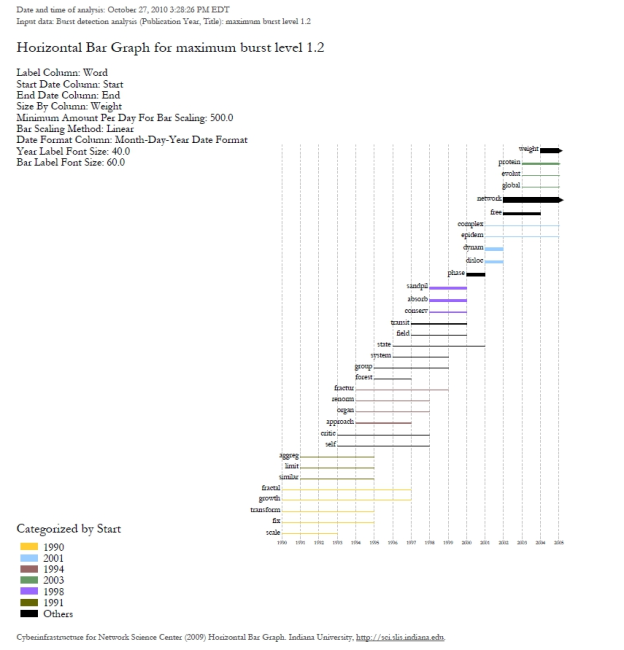
After you manually add this information, save this .csv file somewhere in your computer. Reload this .csv file into Sci2 using 'File > Load'. Select 'Standard csv format' int the pop-up window. A new table will appear in the Data Manager. To visualize these table that contains these new results for the Burst Detection algorithm, select the table you just loaded in the Data Manager and run 'Visualization > Temporal > Horizontal Bar Graph (not included version)' with the same parameters.
A new PostScript file containing the horizontal bar graph will appear in the Data Manager. Once more, open and view the file using the workflow from Section 2.4 Saving Visualizations for Publication.

As expected, a larger number of bursts appear, and the new bursts have a smaller weight that those depicted in the first graph. These smaller, more numerous bursting terms permit a more detailed view of the dataset and allow the identification of trends. The "protein" burst starting in 2003, for example, indicates the year in which Alessandro Vespignani started to work with "protein-protein interaction networks," while the burst "epidem" - also from 2001 - is related to the application of complex networks to the analysis of epidemic phenomena in biological networks.
5.2.5.2 Updating the Vespignani Dataset
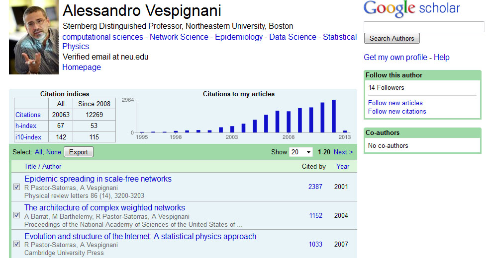
The original dataset for Alessandro Vespignani was created in 2006. If you wish to update the dataset to gain an understanding for how his research has changed and evolved since 2006 you can obtain a new dataset from the from Web of Science, see 4.2.1.3 ISI Web of Science. However, another way to obtain an individual researcher's publication information is to use their Google Scholar profile, if they have one. One of the biggest benefits to using a Google Scholar profile is that you will get publications not indexed in Web of Science, such as some book chapters. In this example, we will obtain the publication information for Alessandro Vespignani using Google Scholar:
Open Google Scholar in a web browser and search for "Alessandro Vespignani":

If the author or investigator you have searched for a Google Scholar profile, you will see a link to their profile at the top of the results page:
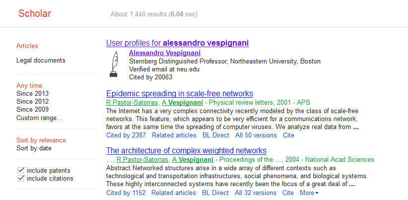
Keep in mind that not every author you search will necessarily have a Google Scholar profile, but for those that do, this is a very useful way to get their publication information. Click on the link to view Alessandro Vespignani's profile, and then select all publications and click the export button at the top of his publication list to export the citation information:
The easiest way to import the citation data into Sci2 is to export the data as a CSV file:
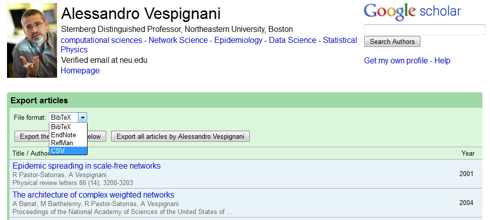
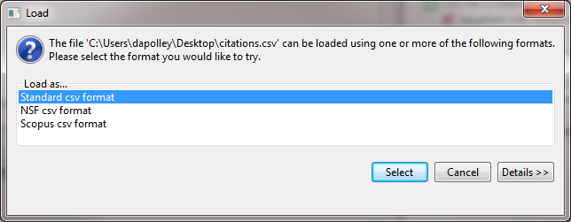
After you have specified the export format you can save the CSV file to your desired location by clicking the "Export all articles by Alessandro Vespignani" button. Save the file to your desktop and then load it into Sci2 in the standard CSV format:
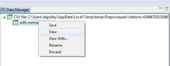
Once the data is in Sci2, you will need to normalize the text for the titles before you can run Burst Detection. Run 'Preprocessing > Topical > Lowercase, Tokenize, Stem, and Stopword Text' and select the title parameter:

After you normalize the text for the title field you will notice a "with normalized Title" file in the data manager. You will likely need to edit this file before you can run Burst Detection. Right click on the file in the data manager and select view:
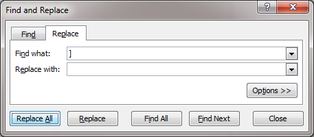
This will open the dataset in Excel (or you preferred spreadsheet editor). You will notice that the Lowercase, Tokenize, Stem, and Stopword Text algorithm has place brackets around the years. You will need to remove these before you can run the Burst Detection algorithm. In Excel, hit 'Ctrl-F' on the keyboard. This will bring up the Find and Replace tool. Highlight the column of years and then perform a find and replace:
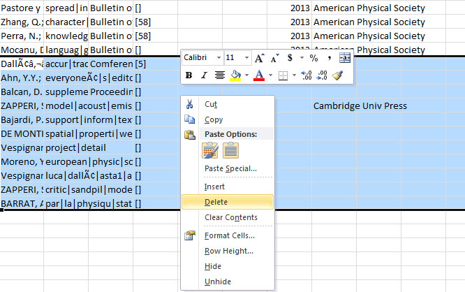
You will have to repeat this for the other bracket symbol. This will essentially allow you remove the brackets around the years. Next you will need to remove those publications for which there is no year information. Burst Detection will not run if there are empty values in the date column. You can search for the publications and find the proper date, but the year value could be empty because these are forthcoming publications. In this example, we will just remove all publications without a value in the year column:
You will need to save this file to your desktop and re-load it into Sci2. Then, select the file you have just loaded and run 'Analysis > Topical > Burst Detection' and enter the following parameters:
This will result in a "Burst detection analysis (Year, Title): maximum burst level 1" file in the data manager Right click on this file to view the data:
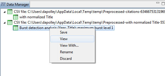
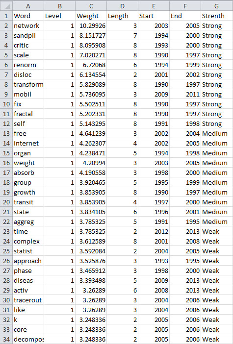
You will need to edit the data before you can run the Temporal Bar Graph algorithm to visualize the results of the burst detection. First, you should make sure every record has an "End" date or the Temporal Bar Graph will not run properly. We know that this dataset contains records that are labeled with the year of 2013, so that will be our end date for those bursts that are still continuing:
Before you can visualize the results with the Temporal Bar Graph it is important to know that if you want to size bars based on weight, the weight value will be distributed across the length of the burst. In other words, the total area of the bar corresponds to the weight value. This means you can have a bar with a high weight value that appears thinner, compared to bar with a lower weight value if the former burst occurs over a longer period than the latter. Finally, before you visualize this dataset, you can add some categories to allow you to color your bars. For example you can sort the records from largest to smallest based on the "total weight" column and assign strong, medium, and weak categories to these records based on the "total weight" values:
Now, save the file to your desktop and reload it into Sci2 in the standard CSV format and run 'Visualization > Temporal > Temporal Bar Graph', entering the following parameters:
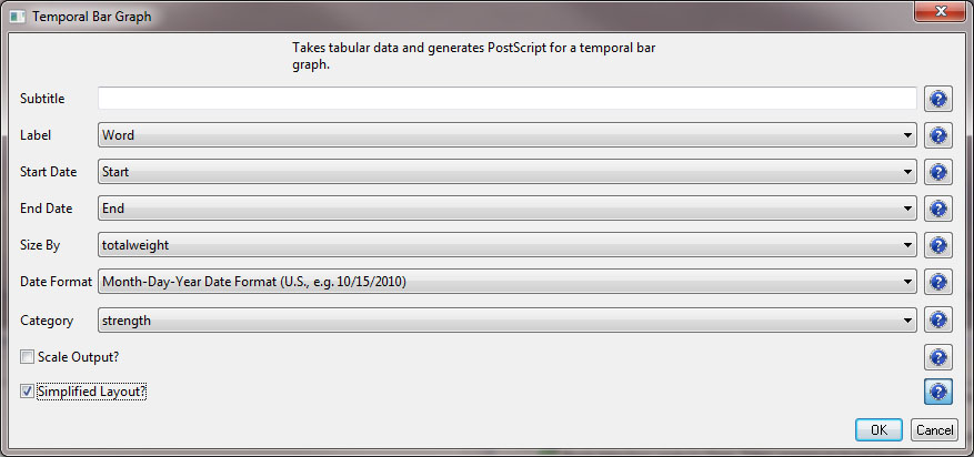
Note that if you select the "Simplified Layout" option no legend will be created for the map. This allows you to create your own legend that will be accurate based creating new weight values. To learn how to create a legend for your visualization see 2.4 Saving Visualizations for Publication.
To view the visualization, save the file from the data manager by right-clicking and selecting save:
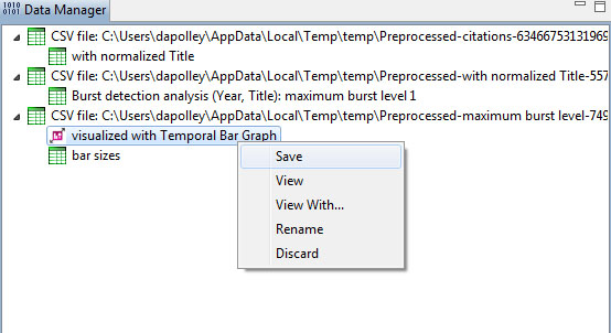
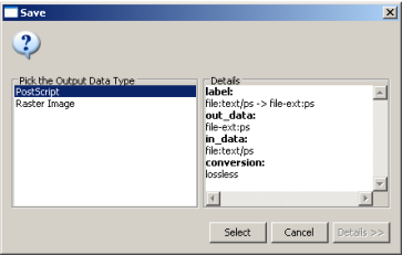
Make sure to save the visualization as a PostScript file:
Save the PostScript file to your desktop, and if you have a version of the Adobe Creative Suite on your machine you can simply double-click the PostScript file to launch Adobe Distiller and automatically convert the PostScript file into a PDF for viewing. However, if you do not have a copy of the Adobe Creative Suite installed on your machine, you can use an online version of GhostScript to convert PostScript files to PDF files: http://ps2pdf.com/. The resulting visualization should look similar to the following:

Remember that the weight for the bars is equal to the total area, not simply the thickness. So, including the color categories will help users make more sense of the visualization. You notice that this burst analysis for Alessandro Vesipignani's publications looks similar to the one created in the previous section. However, this new burst analysis takes into consideration his more recent publications and interests in human mobility networks and epidemiology. This workflow can easily be repeated using any author who has a profile in Google Scholar. Give it a try for yourself!
5.2.5.3 Visualizing Burst Detection in Excel
Its possible to generate a visualization for burst analysis in MS Excel. For this, open the results of the first burst analysis conducted ('Burst detection analysis (Publication Year, Title): maximum burst level 1') in MS Excel, by right clicking on this table in the Data Manager and selecting View.
To generate a visual depiction of the bursts in MS Excel perform the following steps:
1. Sort the data ascending by burst start year.
2. Add column headers for all years, i.e., enter first the start year in the cell of index G1, here 1990. As stated before, when there is no value in the "End" field that indicates that the burst lasted until the last date present in the dataset. So continue, e.g., using formula '=G1+1', until highest burst end year, here 2006 in cell W1.
3. In the resulting word by burst year matrix, select the upper left blank cell (G2) and select 'Conditional Formatting' from the ribbon. Then select 'Data Bars > More Rules > Use a formula to determine which cells to format.' To color cells for years with a burst weight value of more or equal 10 red and cells with a higher value dark red use the following formulas and format patterns:
=AND(AND(G$1>=$E2,OR(G$1<=$F2,$F2="")),$C2>=10)

Select 'OK' and then repeat step three, using the formula below:
=AND(G$1>=$E2,OR(G$1<=$F2,$F2=""))

4. Once both formatting rules have been established, select 'Conditional Formatting > Manage Rules', highlight the first formatting rule and move to the top of the list:
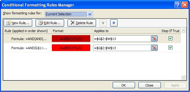
5. Make sure both formatting rules are selected and apply them to current selection. Apply the format to all cells in the word by year matrix by dragging the box around cell G2 to highlight all cells in the matrix. The result for the given example is shown in Figure 5.33
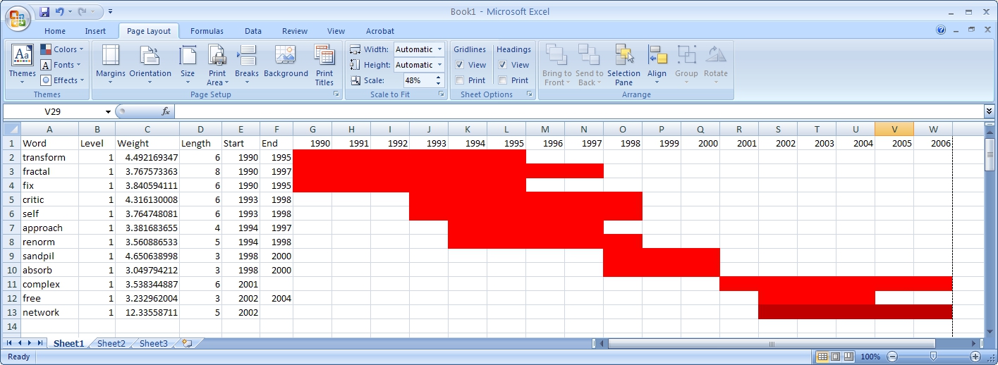
Figure 5.32.1: Visualizing burst results in MS Excel
5.2.6 Mapping the Field of RNAi Research (SDB Data)
RNAi |
|
Time frame: | 1865-2008 |
Region(s): | Miscellaneous |
Topical Area(s): | RNAi |
Analysis Type(s): | Co-Author Network, Patent-Citation Network, Burst Detection |
The database plugin is not currently available for the most recent version of Sci2 (v1.0 aplpha). However, the plugin that allows files to be loaded as databases is available for Sci2 v0.5.2 alpha or older. Please check the Sci2 news page (https://sci2.cns.iu.edu/user/news.php). We will update this page when a database plugin becomes available for the latest version of the tool.
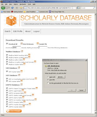
The data for this analysis comes from a search of the Scholarly Database (SDB) (http://sdb.cns.iu.edu/) for "RNAi" in "All Text" from Medline, NSF, NIH and USPTO. A copy of this data is available in 'yoursci2directory/sampledata/scientometrics/sdb/RNAi' (if the file is not in the sample data directory it can be downloaded from 2.5 Sample Datasets). The default export format is .csv, which can be loaded directly into the Sci2 Tool.
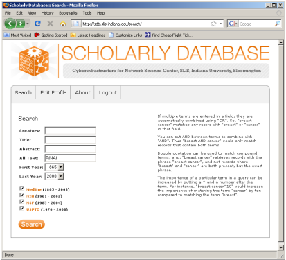

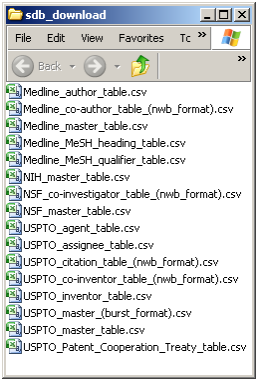
Figure 5.33: Downloading and saving RNAi data from the Scholarly Database.
To view the co-authorship network of Medline's RNAi records, go to 'File > Load' and open 'yoursci2directory/sampledata/scientometrics/sdb/RNAi/Medline_co-author_table(nwb_format).csv'_ in Standard csv format (if the file is not in the sample data directory it can be downloaded from 2.5 Sample Datasets). SDB tables are already normalized, so simply run 'Data Preparation > Extract Co-Occurrence Network' using the default parameters:
According to 'Analysis > Networks > Network Analysis Toolkit (NAT)', the output network has 21,578 nodes with 131 isolates, and 77,739 edges. Visualizing such a large network is memory-intensive, so extract only the largest connected component by running 'Analysis > Networks > Unweighted and Undirected > Weak Component Clustering' with the following parameters:
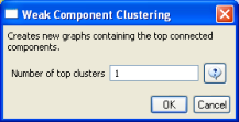
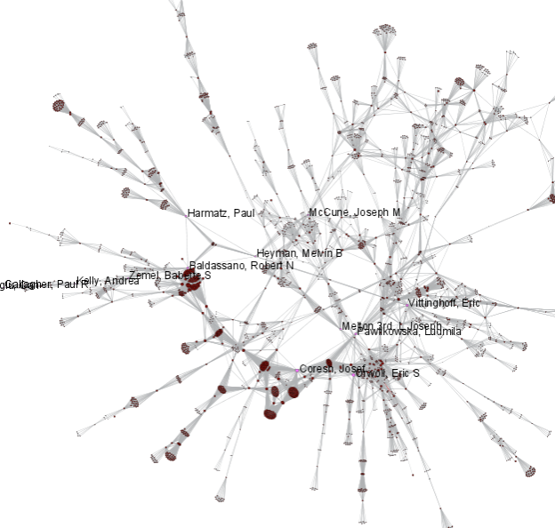
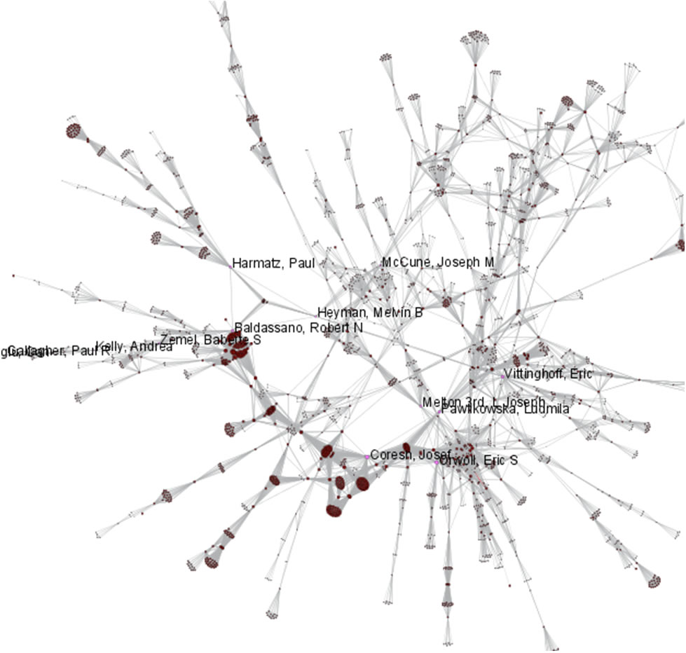
Make sure the newly extracted network ("Weak Component Cluster of 6446 nodes") is selected in the data manager, and run 'Visualization > Networks > GUESS' followed by 'Layout > GEM'. A custom python script has been used to color and size the network in Figure 5.34.
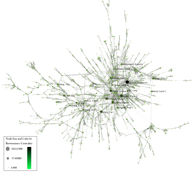
Figure 5.34: The Medline RNAi Co-authorship Network
To visualize the citation patterns of patents dealing with RNAi, load 'yoursci2directory/sampledata/scientometrics/sdb/RNAi/USPTO_citation_table(nwb_format).csv'_ in Standard csv format (if the file is not in the sample data directory it can be downloaded from 2.5 Sample Datasets). Then run 'Data Preparation > Extract Bipartite Network' using the following parameters:

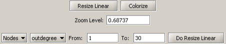
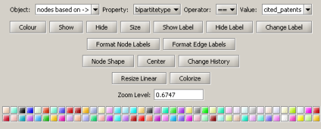
Run 'Analysis > Networks > Unweighted & Directed > Node Indegree' to append Indegree attributes to each node, and then visualize "Network with indegree attribute added to node list" using 'Visualization > Networks > GUESS' followed by 'Layout > GEM' and 'Layout > Bin Pack'. In the graph modifier pane, use the following parameters and click "Do Resize Linear."
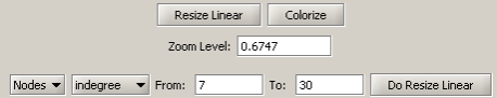
Then select "nodes based on ->" in the Object drop-down box, "bipartitetype" in the Property drop-down box, "==" in the Operator drop-down box, and "cited_patents" in the Value drop-down box. Press "Colour" and click on blue below.

Repeat the previous steps, but change the Value to "citing_patent" and select the color red. Now press "Show Label". The resulting graph should look like Figure 5.35.
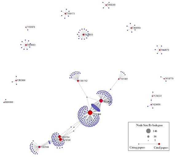
Figure 5.35: USPTO Patent citation network on RNAi
The SDB also outputs much more robust tables, for example 'yoursci2directory/sampledata/scientometrics/sdb/RNAi/Medline_master_table.csv'. This table includes full records of Medline papers, and will be used to find bursting terms from Medline abstracts dealing with RNAi. You can download the file by clicking here.
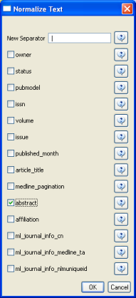
Load the file in Standard csv format and run 'Preprocessing > Topical > Lowercase, Tokenize, Stem, and Stopword Text' with the following parameters:
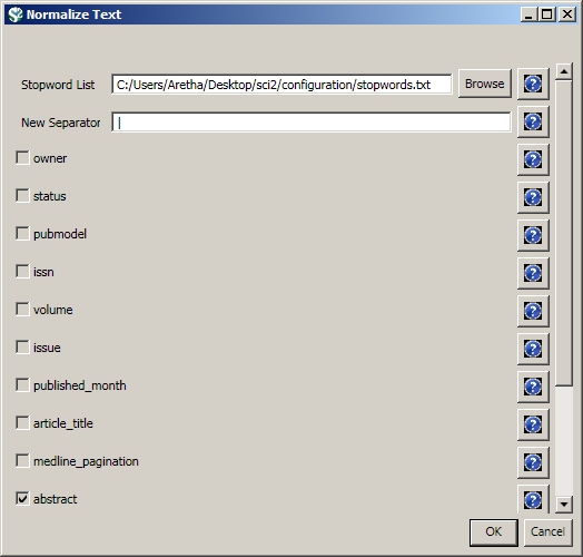
Select the "with normalized abstract" table in the Data Manager and run 'Analysis > Topical > Burst Detection' with the following parameters:
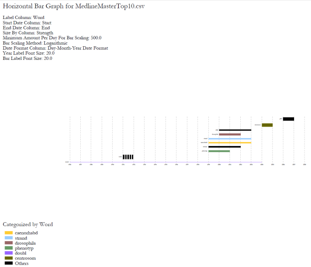
View the file "Burst detection analysis (date_cr_year, abstract): maximum burst level 1." There are more words than can easily be viewed with the horizontal bar graph, so sort the list by "Strength" and prune all but the strongest 10 words. In other words save the file from the data manager and sort the file by the weight column. Delete all but the top 10 rows. Save the file as a new .csv and load it into the Sci2 Tool as a standard csv file.
Select the new table in the data manager and visualize it using 'Visualize > Temporal > Horizontal Bar Graph (not included version)Temporal Bar Graph' with the following parameters:

Save and view the resulting PostScript file using the workflow described in section 2.4 Saving Visualizations for Publication.
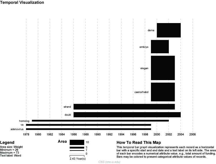
Figure 5.36: Top ten burst terms from Medline abstracts on RNAi Global Level Studies – Meso
To see the log file from this workflow save the 5.2.6 Mapping the Field of RNAi Research (SDB Data) log file.