The study of networks aims to increase our understanding of natural and man-made networks. It builds on social network analysis, physics, information science, bibliometrics, scientometrics, econometrics, informetrics, webometrics, communication theory, sociology of science, and several other disciplines.
Authors, institutions, and countries, as well as words, papers, journals, patents, and funding are represented as nodes and their complex interrelations as edges. Nodes and edges can have (time-stamped) attributes.
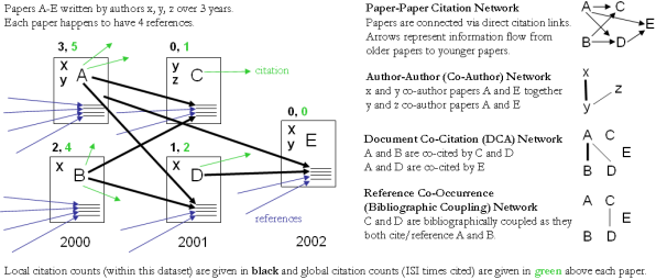
Figure 4.12 shows a sample dataset of five papers, A through E, published over three years together with their authors' x, y, z, references (blue references are papers outside this set) and citations (green ones go to papers outside this set) as well as some commonly derived networks. The extraction and analysis of these and other scholarly networks is explained subsequently.

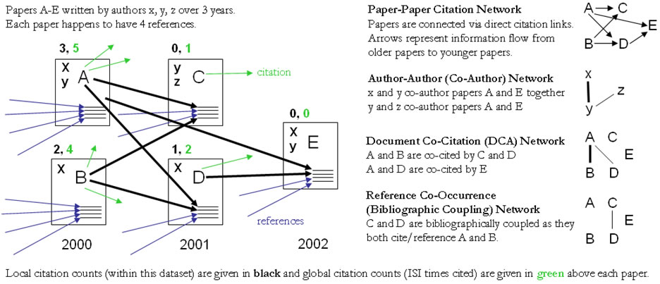
Figure 4.12: Sample paper network (left) and four different network types derived from it (right)

Diverse algorithms exist to calculate specific node, edge, and network properties. Node properties comprise degree centrality, betweenness centrality, or hub and authority scores. Edge properties include durability, reciprocity, intensity (weak or strong), density (how many potential edges in a network actually exist), reachability (how many steps it takes to go from one "end" of a network to another), centrality (whether a network has a "center" point), quality (reliability or certainty), and strength. Network properties refer to the number of nodes and edges, network density, average path length, clustering coefficient, and distributions from which general properties such as small-world, scale-free, or hierarchical can be derived. Identifying major communities via community detection algorithms and calculating the "backbone" of a network via pathfinder network scaling or maximum flow algorithms helps to communicate and make sense of large scale networks.

4.9.1 Network Extraction

4.9.1.1 Direct Linkages

4.9.1.1.1 Document-Document (Citation) Network

Papers cite other papers via references forming an unweighted, directed paper citation graph. It is beneficial to indicate the direction of information flow, in order of publication, via arrows. Such a representation allows for the tracking of citation networks chronologically, yielding a better understanding of the influence of previous research on subsequent research, which more clearly describes the scholarly relationship between individual publications. Citations to a paper support the forward traversal of the graph. Citing and being cited can be seen as roles a paper possesses (Nicolaisen, 2007).

4.9.1.1.2 Author-Author (Citation) Network

Authors cite other authors via document references forming a weighted, directed author citation graph. Like document-document networks, author citation networks represent the flow of information over time. Unlike document citations, however, these networks have weighted edges representing the volume of citations from one author to the next.

4.9.1.1.3 Source-Source (Citation) Network

For larger scale studies, it is often useful to explore citation patterns between entire journals and other varieties of publications. These networks can reveal both the relative importance of certain publications, and the underlying connections between disciplines. These networks are directed and weighted by volume of citations between journals.

4.9.1.1.4 Author-Paper (Consumed/Produced) Network

There are active and passive units of science. Active units, e.g., authors, produce and consume passive units, e.g., papers, patents, datasets, software. The resulting networks have multiple types of nodes, e.g., authors and papers. Directed edges indicate the flow of resources from sources to sinks, e.g., from an author to a written/produced paper to the author who reads/consumes the paper.

4.9.1.2 Co-Occurrence Linkages

4.9.1.2.1 Author Co-Occurrence (Co-Author) Network

Having the names of two authors (or their institutions, countries) listed on one paper, patent, or grant is an empirical manifestation of scholarly collaboration. The more often two authors collaborate, the higher the weight of their joint co-author link. Weighted, undirected co-authorship networks appear to have a high correlation with social networks that are themselves impacted by geospatial proximity (Börner, Penumarthy, Meiss, & Ke, 2006; Wellman, White, & Nazer, 2004).

4.9.1.2.2 Document Cited Reference Co-Occurrence (Bibliographic Coupling) Network

Papers, patents or other scholarly records that share common references are said to be coupled bibliographically (Kessler, 1963),

Figure 4.13: An example of a bibliographic coupling network

The bibliographic coupling (BC) strength of two scholarly papers can be calculated by counting the number of times that they reference the same third work in their bibliographies. The coupling strength is assumed to reflect topic similarity. Co-occurrence networks are undirected and weighted.

4.9.1.2.3 Author Cited Reference Co-Occurrence (Bibliographic Coupling) Network

Authors who cite the same sources are coupled bibliographically. The bibliographic coupling (BC) strength between two authors can be said to be a measure of similarity between them. The resulting network is weighted and undirected.

4.9.1.2.4 Journal Cited Reference Co-Occurrence (Bibliographic Coupling) Network

Like document and author bibliographic coupling networks, journal cited reference co-occurrences provide a measurement of similarity between journals. Edge strength between two journals is determined by summing the number of unique references both journals cite.

4.9.1.3 Co-Citation Linkages

Two scholarly records are said to be co-cited if they jointly appear in the list of references of a third paper. The more often two units are co-cited the higher their presumed similarity.

4.9.1.3.1 Document Co-Citation Network (DCA)

DCA was simultaneously and independently introduced by Small and Marshakova in 1973 (Marshakova, 1973; Small, 1973; Small & Greenlee, 1986). It is the logical opposite of bibliographic coupling. The co-citation frequency equals the number of times two papers are cited together, i.e., they appear together in one reference list.

4.9.1.3.2 Author Co-Citation Network (ACA)

Authors of works that repeatedly appear together in lists of references are assumed to be related. Clusters in ACA networks often reveal shared schools of thought or methodology, common subjects of study, collaborative and student-mentor relationships, ties of nationality, etc. Some regions of scholarship are densely crowded and interactive. Others are isolated or nearly vacant.

4.9.1.3.3 Journal Co-Citation Network (JCA)

JCA networks offer wide-angle views of scholarly disciplines. Slicing these networks by time can reveal the evolution of disciplinary similarity. Like author and document co-citation networks, these are undirected and weighted.

4.9.2 Compute Basic Network Characteristics

It is often advantageous to know for a network

• Whether it is directed or undirected
• Number of nodes
• Number of isolated nodes
• A list of node attributes
• Number of edges
• Whether the network has self loops, if so, lists all self loops
• Whether the network has parallel edges, if so, lists all parallel edges
• A list of edge attributes
• Average degree
• Whether the graph is weakly connected
• Number of weakly connected components
• Number of nodes in the largest connected component
• Strong connectedness for directed networks
• Graph density

In the Sci2 Tool, use 'Analysis > Network Analysis Toolkit (NAT)' to get basic properties, e.g., for the network of
Florentine families available in 'yoursci2directory/sampledata/socialscience/florentine.nwb'. The result for this dataset is:

     This graph claims to be undirected.
     Nodes: 16
     Isolated nodes: 1
     Node attributes present: label, wealth, totalities, priorates
     Edges: 27
     No self loops were discovered.
     No parallel edges were discovered.
     Edge attributes:
     Nonnumeric attributes:
     Example value
     marriag[tab] T
     busines[tab] F
     Did not detect any numeric attributes
     This network does not seem to be a valued network.
     Average degree: 3.375
     This graph is not weakly connected.
     There are 2 weakly connected components. (1 isolates)
     The largest connected component consists of 15 nodes.
     Did not calculate strong connectedness because this graph was not directed.
     Density (disregarding weights): 0.225

4.9.3 Network Analysis

In the analysis menu, certain algorithms append values to each node, or delete groups of nodes and edges entirely:

• Weak Component Clustering extracts the N largest weakly connected components of a network
• Node Degree calculates the number of edges adjacent to a node
• Pathfinder Network Scaling prunes a network to find its underlying structure
• Node Betweenness Centrality appends a value to each node which correlates to the number of shortest paths that node resides on. The more "shortest paths" between node-pairs a certain node resides on, the higher its betweenness centrality. To learn about each algorithm, see section 3.1 'Sci2 Tool Plugins' or visit https://nwb.cns.iu.edu/community/ for greater detail.

4.9.4 Network Visualization

4.9.4.1 GUESS Visualizations

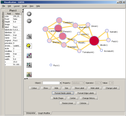
Load the sample dataset 'yoursci2directory/sampledata/socialscience/florentine.nwb' and calculate an additional node attribute 'Betweenness Centrality' by running 'Analysis > Networks > Unweighted and Undirected > Node Betweenness Centrality' with default parameters. Then select the network and run 'Visualization > Networks > GUESS' to open GUESS with the file loaded. It might take some time for the network to load. The initial layout will be random. Wait until the random layout is completed and the network is centered before proceeding.
The GUESS window is divided into three sections:

1. Information - Examine node and edge attributes, see Figure 4.14, left
2. Visualization - View and manipulate network, see Figure 4.14, top right.
3. Interpreter/Graph Modifier - Analyze/change network properties, see figure 4.14, bottom right.

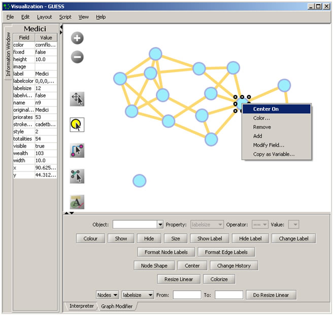
Figure 4.14: GUESS 'Information Window', visualization window, and 'Graph Modifier' window

4.9.4.1.1 Network Layout and Interaction

GUESS provides different network layout algorithms under menu item 'Layout'. Apply 'Layout > GEM' to the Florentine network. Use 'Layout > Bin Pack' to compact and center the network layout. These layout algorithms often employ some degree of randomness, and layouts may look different every time they are used. Also note that running GEM and/or Bin Pack on the same network multiple times will continue to change the visualization each and every time they are used.
Using the mouse pointer, hover over a node or edge to see its properties in the Information window. GUESS has several methods of interaction:

• Pan – simply 'grab' the background by clicking and holding down the left mouse button, and move it using the mouse.
• Zoom – Using the scroll wheel on the mouse OR press the "+" and "-" buttons in the upper-left hand corner of the visualization window OR right-click and move the mouse left or right. Center graph by selecting 'View > Center'.
• Click to select/move single nodes. Hold down 'Shift' to select multiple.
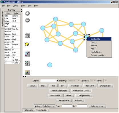
• Right click: Right clicking on a node gives the options to 'Center on', 'Color', 'Toggle Label', 'Remove', 'Add', 'Modify Field', and 'Copy as Variable', see Figure 4.14.

Use the Graph Modifier to change node attributes, e.g.,

• Select 'all nodes' in the Object drop-down menu and click 'Show Label' button.
• Select 'Resize Linear' and choose 'Nodes' and 'totalities' from the drop-down menus. Enter the parameters 'From: 5 To: 20.' Then select 'Do Resize Linear.'
• Select 'Colorize' and choose 'Nodes' and ' totalities' from the drop-down menus. Click the small box next to 'From' and in the pop-up 'Choose the First Color' window, under the 'Swatches' tab, select white, and set the color options under the 'RGB' tab to: (204,0,51) Click 'OK' and then click 'Do Colorize' In the Graph Modifier.
• To view the entities associated with each node, click the 'Show Label' button. To modify node labels, select 'Format Node Labels,' and replace the default text with your own label in the pop-up box . The labels shown in Figure 4.15 have been modified to '{originallabel and '.

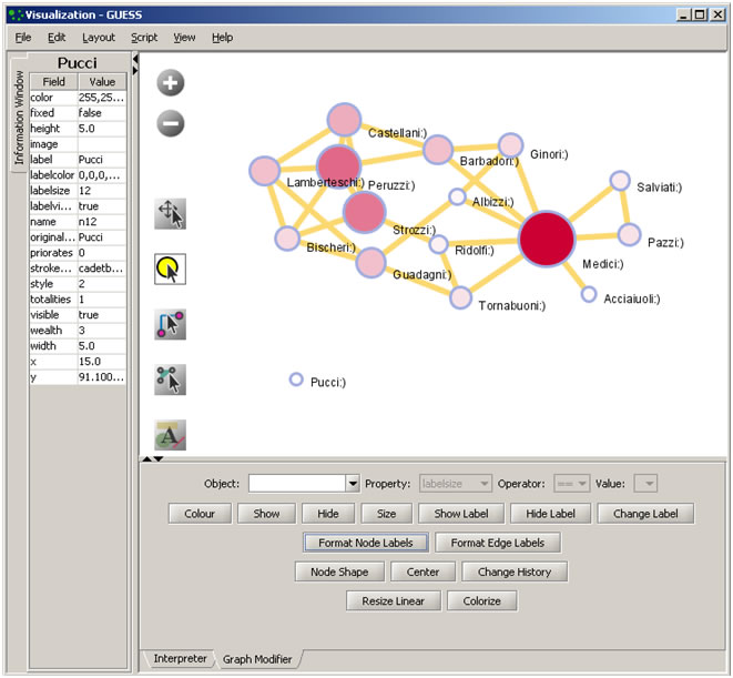
Figure 4.15: Using the GUESS 'Graph Modifier'

4.9.4.1.2 Interpreter

Use Jython, a version of Python that runs on the Java Virtual Machine, to write code in the interpreter. Here we list some GUESS commands which can be used to modify the layout.
Color all nodes uniformly
     g.nodes.color =red
     g.nodes.strokecolor =red
     g.nodes.labelcolor =red
     colorize(numberofworks,gray,black)
     for n in g.nodes:
          n.strokecolor = n.color

Size code nodes
     g.nodes.size = 30
     resizeLinear(numberofworks,.25,8)

Label
     for n in g.nodes:
n.labelvisible = true
Print
for n in g.nodes:
print n.label + ":" + str(n.indegree)
Edges
g.edges.width=10
g.edges.color=gray
Color and resize nodes based on their betweenness:
colorize(wealth,white,red)
resizeLinear(sitebetweenness,5,20)

The result is shown in Figure 4.16. Read https://nwb.cns.iu.edu/community/?n=VisualizeData.GUESS for more information on how to use the interpreter.

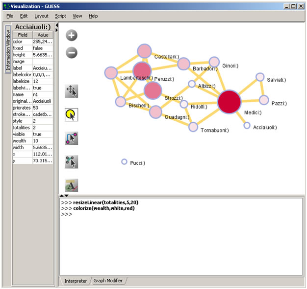
Figure 4.16: Using the GUESS 'Interpreter'

4.9.4.2 DrL Large Network Layout

DrL is a force-directed graph layout toolbox for real-world large-scale graphs up to 2 million nodes (Davidson, Wylie, & Boyack, 2001; Martin, Brown, & Boyack,unpublished). It includes:

• Standard force-directed layout of graphs using an algorithm based on the popular VxOrd routine (used in the VxInsight program).
• Parallel version of force-directed layout algorithm.
• Recursive multilevel version for obtaining better layouts of very large graphs.
• Ability to add new vertices to a previously drawn graph.

This is one of the few force-directed layout algorithms that can scale to over 1 million nodes, making it ideal for large graphs. However, the algorithm doesn't always render small graphs ( less than a hundred records) well. The algorithm expects similarity matrices as input. Distance and other networks will have to be converted before they can be laid out. For article/citation networks, feed the network into either cocitation or bibliographic coupling for computing similarity. Use this network for laying out DrL.
The version of DrL included in Sci2 only does the standard force-directed layout (no recursive or parallel computation). DrL expects the edges to be weighted, directed edges where the weight (greater than zero) denotes how similar the two nodes are (higher is more similar). The Sci2 version has several parameters. The edge cutting parameter expresses how much automatic edge cutting should be done. 0 means as little as possible, 1 as much as possible. Around .8 is a good value to use. The weight attribute parameter lets users choose which edge attribute in the network corresponds to the similarity weight. The X and Y parameters let users choose the attribute names in the returned network which correspond to the X and Y coordinates computed by the layout algorithm for the nodes.
DrL is commonly used to lay out large networks such as co-citation and co-word analyses. In the Sci2 Tool, the results can be viewed in either GUESS or 'Visualization > Specified (prefuse alpha)'. For more information see https://nwb.cns.iu.edu/community/?n=VisualizeData.DrL.
For an application of DrL, see 5.1.4.5 Word Co-Occurrence Network.