- 5.1.4.1 Paper-Paper (Citation) Network
- 5.1.4.2 Author Co-Occurrence (Co-Author) Network
- 5.1.4.3 Cited Reference Co-Occurrence (Bibliographic Coupling) Network
- 5.1.4.4 Document Co-Citation Network (DCA)
- 5.1.4.5 Word Co-Occurrence Network
FourNetSciResearchers.isi |
|
Time frame: | 1955-2007 |
Region(s): | Miscellaneous |
Topical Area(s): | Network Science |
Analysis Type(s): | Paper Citation Network, Co-Author Network, Bibliographic Coupling Network, Document Co-Citation Network, Word Co-Occurrence Network |
5.1.4.1 Paper-Paper (Citation) Network
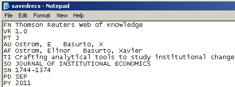
Load the file using 'File > Load' and following this path: 'yoursci2directory/sampledata/scientometrics/isi/FourNetSciResearchers.isi' (if the file is not in the sample data directory it can be downloaded from 2.5 Sample Datasets). A table of all records and a table of 361 records with unique ISI ids will appear in the Data Manager. In this "clean" file, each original record now has a "Cite Me As" attribute that is constructed from the first author, publication year (PY), journal abbreviation (J9), volume (VL), and beginning page (BP) fields of its ISI record. This "Cite Me As" attribute will be used when matching paper and reference records.
New ISI File Format
Web of Science made a change to their output format in September, 2011. Older versions of Sci2 tool (Older than v0.5.2 alpha) may refuse to load these new files, with an error like "Invalid ISI format file selected."
Sci2 solution
If you are using an older version of the Sci2 tool, you can download the WOS-plugins.zip file and unzip the JAR files into your sci2/plugins/ directory. Restart Sci2 to activate the fixes. You can now load the downloaded ISI files into the Sci2 without any additional step. If you are using the old Sci2 tool you will need to follow the guidelines below before you can load the new WOS format file into the tool.
You can fix this problem for individual files by opening them in Notepad (or your favorite text editor). The file will start with the words:
Original ISI file:
Just add the word ISI.
Updated ISI file:
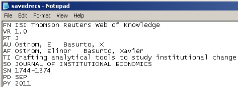
And then Save the file.
The ISI file should now load properly. More information on the ISI file format is available here (http://wiki.cns.iu.edu/display/CISHELL/ISI+%28*.isi%29).
To extract the paper citation network, select the '361 Unique ISI Records' table and run 'Data Preparation > Extract Directed Network' using the parameters :
Aggregate Function File
Make sure to use the aggregate function file indicated in the image below. Aggregate function files can be found in sci2/sampledata/scientometrics/properties.
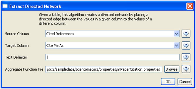
The result is a directed network of paper citations in the Data Manager. Each paper node has two citation counts. The local citation count (LCC) indicates how often a paper was cited by papers in the set. The global citation count (GCC) equals the times cited (TC) value in the original ISI file. Only references from other ISI records count towards an ISI paper's GCC value. Currently, the Sci2 Tool sets the GCC of references to -1 (except for references that are not also ISI records) to prune the network to contain only the original ISI records.
To view the complete network, select the "Network with directed edges from Cited References to Cite Me As" in the Data Manager and run 'Visualization > Networks > GUESS' and wait until the network is visible and centered. Because the FourNetSciResearchers dataset is so large, the visualization will take some time to load, even on powerful systems.
Select ' Layout > GEM' to group related nodes in the network. Again, because of the size of the dataset, this will take some time. Use 'Layout > Bin Pack' to "pack" the nodes and edges, bringing them closer together for easier analysis and comparison. To size and color-code nodes in the "Graph Modifier," use the following workflow:
- Resize Linear > Nodes > globalcitationcount> From: 1 To: 50 > When the nodes have no 'globalcitationcount': 0.1 > Do Resize Linear
- Colorize > Nodes > globalcitationcount > From:
 To:
To:  (When the nodes have no 'globalcitationcount': 0.1 >
  >Do Colorize)
 - Colorize > Edges > weight > From (select the "RGB" tab) 127, 193, 65 To: (select the "RGB" tab) 0, 0, 0
- Type in Interpreter:
>for n in g.nodes:
     n.strokecolor = n.color
Or, select the 'Interpreter' tab at the bottom, left-hand corner of the GUESS window, and enter the command lines:
> resizeLinear(globalcitationcount,1,50)
> colorize(globalcitationcount,gray,black)
> for e in g.edges:
      e.color="127,193,65,255"
Note: The Interpreter tab will have '>>>' as a prompt for these commands. It is not necessary to type '>" at the beginning of the line. You should type each line individually and press "Enter" to submit the commands to the Interpreter.
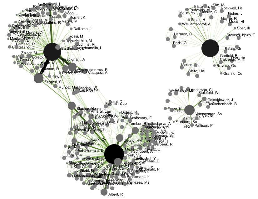
This will result in nodes which are linearly sized and color coded by their GCC, connected by green directed edges, as shown in Figure 5.11 (left). Any numeric node attribute within the network can be used to code the nodes. To view the available attributes, mouse over a node. The GUESS interface supports pan and zoom, node selection, and details on demand. For more information, refer to the GUESS tutorial at http://nwb.cns.iu.edu/Docs/GettingStartedGUESSNWB.pdf
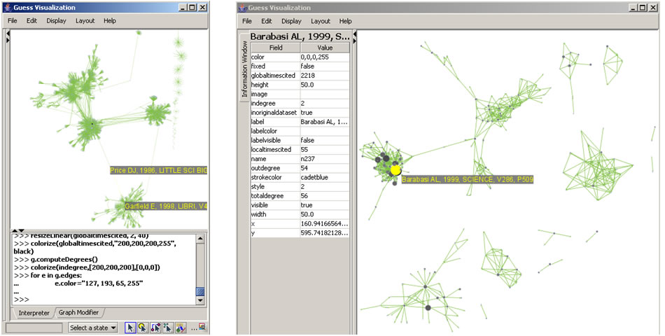
Figure 5.11: Directed, unweighted paper-paper citation network for 'FourNetSciResearchers' dataset with all papers and references in the GUESS user interface (left) and a pruned paper-paper citation network after removing all references and isolates (right)
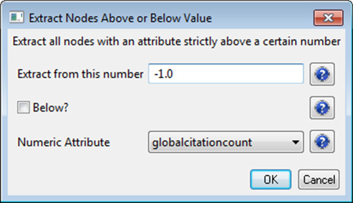
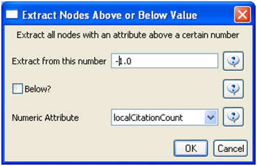
The complete network can be reduced to papers that appeared in the original ISI file by deleting all nodes that have a GCC of -1. Simply run 'Preprocessing > Networks > Extract Nodes Above or Below Value' with parameter values:
The resulting network is unconnected, i.e., it has many subnetworks many of which have only one node. These single unconnected nodes, also called isolates, can be removed using 'Preprocessing > Networks > Delete Isolates'. Deleting isolates is a memory intensive procedure. If you experience problems at this step, refer to Section 3.4 Memory Allocation.
The 'FourNetSciResearchers' dataset has exactly 65 isolates. Removing those leaves 12 networks shown in Figure 5.11 (right) using the same color and size coding as in Figure 5.11 (left). Using 'View > Information Window' in GUESS reveals detailed information for any node or edge.
Alternatively, nodes could have been color and/or size coded by their degree using, e.g.:
> g.computeDegrees()
> colorize(outdegree,gray,black)
Note that the outdegree corresponds to the LCC within the given network while the indegree reflects the number of references, helping to visually identify review papers.
The complete paper-paper-citation network can be split into its subnetworks using 'Analysis > Networks > Unweighted & Directed > Weak Component Clustering' with the default values:
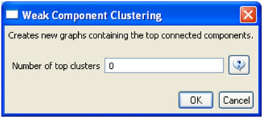
The largest component has 2407 nodes; the second largest, 307; the third, 13; and the fourth has 7 nodes. The largest component is shown in Figure 5.12. The top 20 papers, by times cited in ISI, have been labeled using
> toptc = g.nodes[:]
> def bytc(n1, n2):
      return cmp(n1.globalcitationcount, n2.globalcitationcount)
> toptc.sort(bytc)
> toptc.reverse()
> toptc
> for i in range(0, 20):
      toptc[i].labelvisible = true
Alternatively, run 'Script > Run Script' and select 'yoursci2directory/scripts/GUESS/paper-citation-nw.py'.
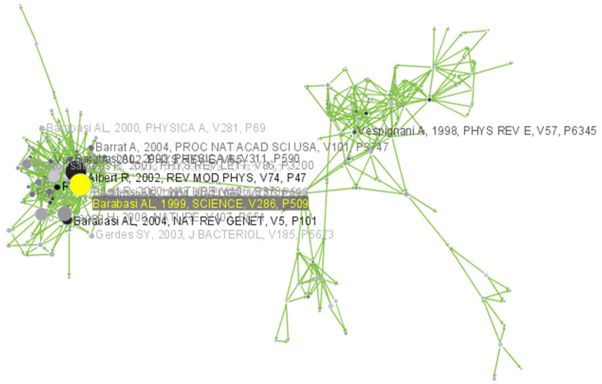
Figure 5.12: Giant components of the paper citation network
Compare the result with Figure 5.11 and note that this network layout algorithm – and most others – are non-deterministic: different runs lead to different layouts. That said, all layouts aim to group connected nodes into spatial proximity while avoiding overlaps of unconnected or sparsely connected sub-networks.
To see the log file from this workflow save the 5.1.4.1 Paper-Paper (Citation) Network log file.
5.1.4.2 Author Co-Occurrence (Co-Author) Network
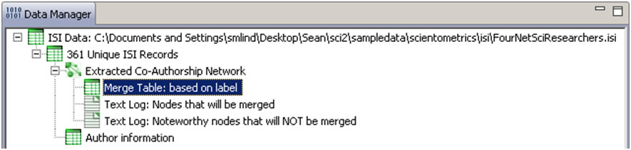
To produce a co-authorship network in the Sci2 Tool, select the table of all 361 unique ISI records from the 'FourNetSciResearchers' dataset in the Data Manager window. Run 'Data Preparation > Extract Co-Author Network' using the parameter:

The result is two derived files in the Data Manager window: the "Extracted Co-Authorship Network" and an "Author information" table (also known as a "merge table"), which lists unique authors. In order to manually examine and edit the list of unique authors, open the merge table in your default spreadsheet program. In the spreadsheet, select all records, including "label," "timesCited," "numberOfWorks," "uniqueIndex," and "combineValues," and sort by "label." Identify names that refer to the same person. In order to merge two names, first delete the asterisk ('*') in the "combineValues" column of the duplicate node's row. Then, copy the "uniqueIndex" of the name that should be kept and paste it into the cell of the name that should be deleted. Resave the revised table as a .csv file and reload it. Select both the merge table and the network and run 'Data Preparation > Update Network by Merging Nodes'. Table 5.2 shows the result of merging "Albet, R" and "Albert, R": "Albet, R" will be deleted and all of the node linkages and citation counts will be added to "Albert, R".
label | timesCited | numberOfWorks | uniqueIndex | combineValues |
Abt, HA | 3 | 1 | 142 | * |
Alava, M | 26 | 1 | 196 | * |
Albert, R | 7741 | 17 | 60 | * |
Albet, R | 16 | 1 | 60 |
|
Table 5.2: Merging of author nodes using the merge table
A merge table can be automatically generated by applying the Jaro distance metric (Jaro, 1989, 1995) available in the open source Similarity Measure Library (http://sourceforge.net/projects/simmetrics/) to identify potential duplicates. In the Sci2 Tool, simply select the co-author network and run 'Data Preparation > Detect Duplicate Nodes'. using the parameters:

The result is a merge table that has the very same format as Table 5.2, together with two textual log files:
The log files describe, in a more human-readable form, which nodes will be merged or not merged. Specifically, the first log file provides information regarding which nodes will be merged, while the second log file lists nodes which are similar but will not be merged. The automatically generated merge table can be further modified as needed.
In sum, unification of author names can be done manually or automatically, independently or in conjunction with other data manipulation. It is recommended that users create the initial merge table automatically and fine-tune it as needed. Note that the same procedure can be used to identify duplicate references – simply select a paper-citation network and run 'Data Preparation > Detect Duplicate Nodes' using the same parameters as above and a merge table for references will be created.
To merge identified duplicate nodes, select both the "Extracted Co-Authorship Network" and "Merge Table: based on label" by holding down the 'Ctrl' key. Run 'Data Preparation > Update Network by Merging Nodes'. This will produce an updated network as well as a report describing which nodes were merged. To complete this workflow, an aggregation function file must also be selected from the pop-up window:
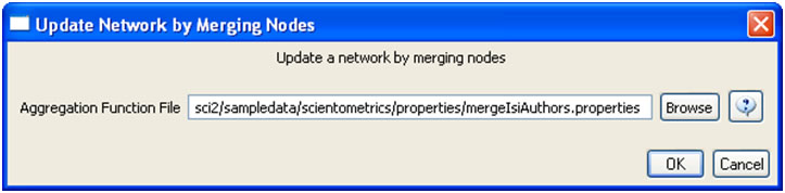
Aggregation files can be found in the Sci2 sample data. Follow this path "sci2/sampledata/scientometrics/properties" and select the mergeIsiAuthors.properties.
The updated co-authorship network can be visualized using 'Visualization > Networks > GUESS', (See section 4.9.4.1 GUESS Visualizations for more information regarding GUESS).
Figure 5.13 shows the layout of the combined 'FourNetSciResearchers' dataset after it was modified using the following commands in the "Interpreter":
> resizeLinear(numberOfWorks,1,50)
> colorize(numberOfWorks,gray,black)
> for n in g.nodes:
      n.strokecolor = n.color
> resizeLinear(numberOfCoAuthored_works, .25, 8)
> colorize(numberOfCoAuthoredworks, "127,193,65,255", black)
> nodesbynumworks = g.nodes[:]
> def bynumworks(n1, n2):
     return cmp(n1.numberofworks, n2.numberofworks)
> nodesbynumworks.sort(bynumworks)
> nodesbynumworks.reverse()
> for i in range(0, 50):
      nodesbynumworks[i].labelvisible = true
Alternatively, run 'Script > Run Script ...' and select ' yoursci2directory/scripts/GUESS/co-author-nw.py'.
For both workflows described above, the final step should be to run 'Layout > GEM' and then 'Layout > Bin Pack' to give a better representation of node clustering.
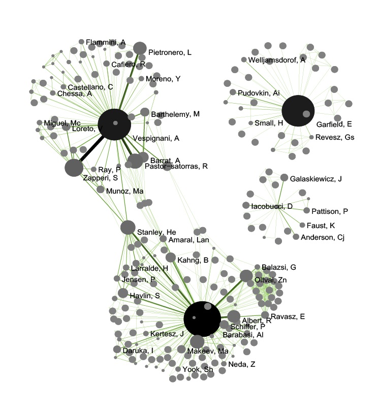
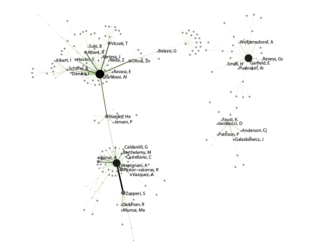
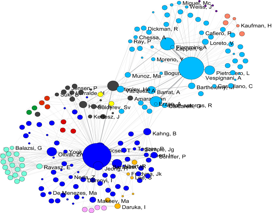
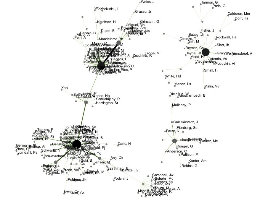
In the resulting visualization, author nodes are color and size coded by the number of papers per author. Edges are color and thickness coded by the number of times two authors wrote a paper together. The remaining commands identify the top 50 authors with the most papers and make their name labels visible.

Figure 5.13: Undirected, weighted co-author network for 'FourNetSciResearchers' dataset
GUESS supports the repositioning of selected nodes. Multiple nodes can be selected by holding down the 'Shift' key and dragging a box around specific nodes. The final network can be saved via 'GUESS: File > Export Image' and opened in a graphic design program to add a title and legend and to modify label sizes. The image above was modified using Photoshop.
Pruning the network
Pathfinder algorithms take estimates of the proximity's between pairs of items as input and define a network representation of the items that preserves only the most important links. The value of Pathfinder Network Scaling for networks lies in its ability to reduce the number of links in meaningful ways, often resulting in a concise representation of clarified proximity patterns.
Given the co-Authorship network extracted at workflow 5.1.4.2, run 'Preprocessing > Networks > Fast Pathfinder Network Scaling' with the following parameters:
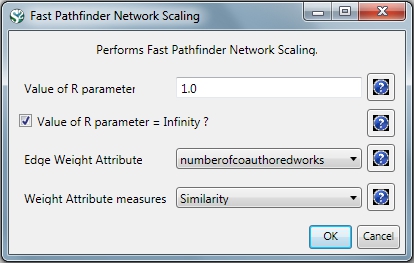
The number of edges reduced from 872 to 731. The updated co-authorship network can be visualized using 'Visualization > Networks > GUESS'.
Inside GUESS, run 'Script > Run Script ...' and select ' yoursci2directory/scripts/GUESS/co-author-nw.py'. Also run 'Layout > GEM' and then 'Layout > Bin Pack' to give a better representation of node clustering. The pruned network looks like this:
If the network being processed is undirected, which is the case, then MST-Pathfinder Network Scaling can be used to prune the networks. This will produce results 30 times faster than Fast Pathfinder Network Scaling. Also, we have found that networks which have a low standard deviation for edge weights, or that have many edge weights that are equal to the minimum edge weight, might not be scaled as much as expected when using Fast Pathfinder Network Scaling. To see this behavior, run 'Preprocessing > Networks > MST-Pathfinder Network Scaling' with the network named 'Updated network' selected with the following parameters:
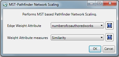
The number of edges reduced from 872 to 235 for the network pruned with the MST-Pathfinder Network Scaling algorithm, while the reduction for the Fast Pathfinder Network Scaling algorithm was from 872 to 731 only.
Visualize this network using 'Visualization > Networks > GUESS'. Inside GUESS, run 'Script > Run Script ...' and select ' yoursci2directory/scripts/GUESS/co-author-nw.py' again. Also run 'Layout > GEM' and then 'Layout > Bin Pack' to give a better representation of node clustering. The pruned network with the algorithm looks like this:
Degree Distribution
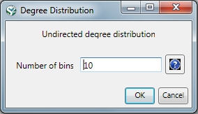
Given the co-Authorship network extracted at workflow 5.1.4.2 (name 'Updated Network' at the Data Manager), run 'Analysis > Networks > Unweighted & Undirected > Degree Distribution' with the following parameter:
This algorithm generates two output files, corresponding to two different ways of partitioning the interval spanned by the values of degree.
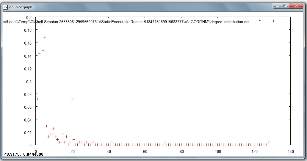
In the first output file named 'Distribution of degree for network at study (equal bins)', the occurrence of any degree value between the minimum and the maximum is estimated and divided by the number of nodes of the network, so to obtain the probability: the output displays all degree values in the interval with their probabilities. Visualize this first output file with 'Visualization > General > GnuPlot':
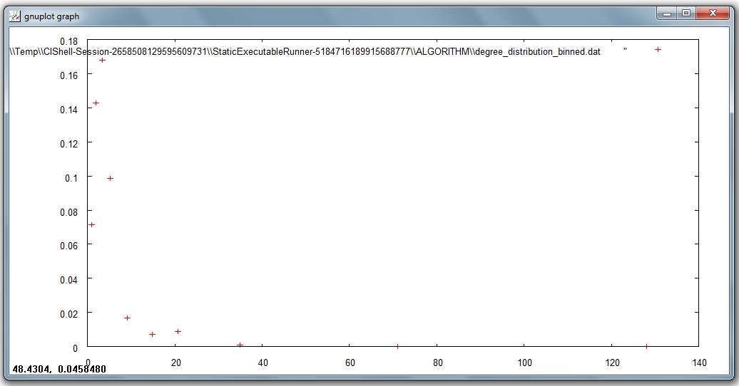
The second output file named 'Distribution of degree for network at study (logarithmic bins)' gives the binned distribution, i.e. the interval spanned by the values of degree is divided into bins whose size grows while going to higher values of the variable. The size of each bin is obtained by multiplying by a fixed number the size of the previous bin. The program calculates the fraction of nodes whose degree falls within each bin. Because of the different sizes of the bins, these fractions must be divided by the respective bin size, to have meaningful averages.
This second type of output file is particularly suitable to study skewed distributions: the fact that the size of the bins grows large for large degree values compensates for the fact that not many nodes have high degree values, so it suppresses the fluctuations that one would observe by using bins of equal size. On a double logarithmic scale, which is very useful to determine the possible power law behavior of the distribution, the points of the latter will appear equally spaced on the x-axis.
Visualize this second output file with 'Visualization > General > GnuPlot':
Community Detection
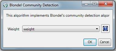
Community Detection algorithms look for subgraphs where nodes are highly interconnected among themselves and poorly connected with nodes outside the subgraph. Many community detection algorithms are based on the optimization of the modularity - a scalar value between -1 and 1 that measures the density of links inside communities as compared to links between communities. The Blondel Community Detection finds high modularity partitions of large networks in short time and that unfolds a complete hierarchical community structure for the network, thereby giving access to different resolutions of community detection.
Run 'Analysis > Networks > Weighted & Undirected > Blondel Community Detection' with the following parameter:
This will generate a network named 'With community attributes' in the Data Manager. To visualize this network run 'Visualization > Networks > Circular Hierarchy' with the following parameters:
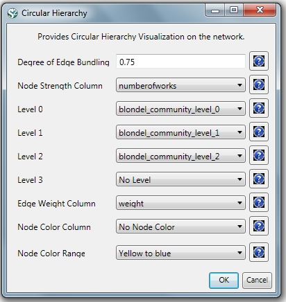
The generated postscript file "CircularHierarchy_With community attributes.ps" can be viewed using Adobe Distiller or GhostViewer (see section 2.4 Saving Visualizations for Publication).
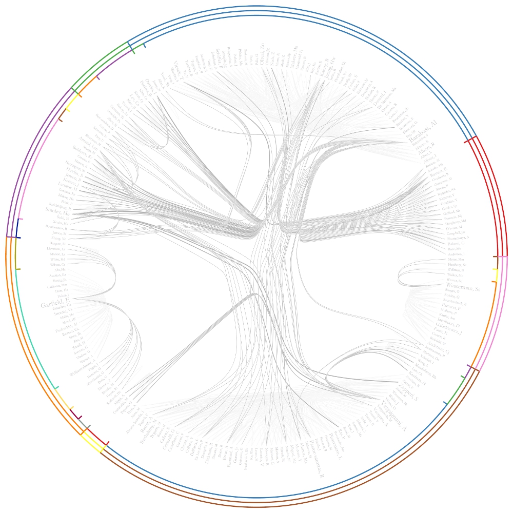
To view to the network with community attributes with in GUESS select the network used to generate the image above and run 'Visualization > Networks > GUESS.'
To see the log file from this workflow save the 5.1.4.2 Author Co-Occurrence (Co-Author) Network log file.
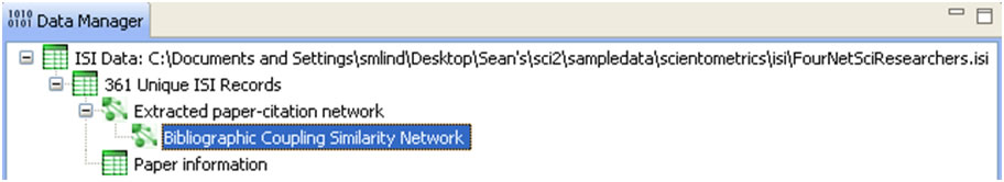
5.1.4.3 Cited Reference Co-Occurrence (Bibliographic Coupling) Network
In Sci2, a bibliographic coupling network is derived from a directed paper citation network (see section 4.9.1.1.1 Document-Document (Citation) Network).
Load the file using 'File > Load' and following this path: 'yoursci2directory/sampledata/scientometrics/isi/FourNetSciResearchers.isi'. A table of all records and a table of 361 records with unique ISI ids will appear in the Data Manager.
Select the "361 Unique ISI Records" in the Data Manager and run 'Data Preparation > Extract Paper Citation Network.' Select "Extracted Paper Citation Network" and run 'Data Preparation > Extract Reference Co-Occurrence (Bibliographic Coupling) Network.'
Running 'Analysis > Networks > Network Analysis Toolkit (NAT)' reveals that the network has 5,342 nodes (5,013 of which are isolate nodes) and 6,277 edges.
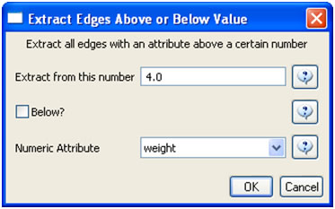
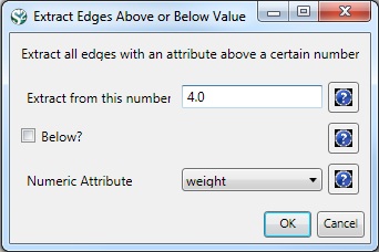
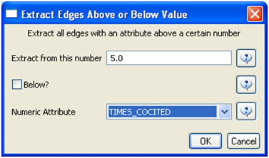
In the "Bibliographic Coupling Similarity Network," edges with low weights can be eliminated by running 'Preprocessing > Networks > Extract Edges Above or Below Value' with the following parameter values:
to produce the following network:
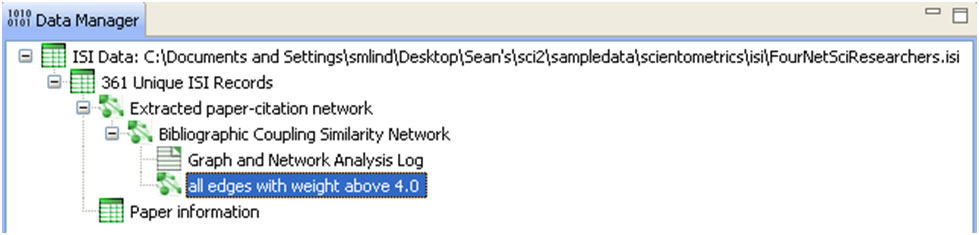
Isolate nodes can be removed running 'Preprocessing > Networks > Delete Isolates'. The resulting network has 242 nodes and 1,534 edges in 12 weakly connected components.
This network can be visualized in GUESS; see Figure 5.14. Nodes and edges can be color and size coded, and the top 20 most-cited papers can be labeled by entering the following lines in the GUESS "Interpreter":
> resizeLinear(globalcitationcount,2,40)
> colorize(globalcitationcount,gray,black)
> resizeLinear(weight,.25,8)
> colorize(weight, "127,193,65,255", black)
> for n in g.nodes:
      n.strokecolor=n.color
> toptc = g.nodes[:]
> def bytc(n1, n2):
      return cmp(n1.globalcitationcount, n2.globalcitationcount)
> toptc.sort(bytc)
> toptc.reverse()
> toptc
> for i in range(0, 20):
      toptc[i].labelvisible = true
Alternatively, run 'GUESS: File > Run Script ...' and select 'yoursci2directory/scripts/GUESS/reference-co-occurence-nw.py'.
For both workflows described above, the final step should be to run 'Layout > GEM' and then 'Layout > Bin Pack' to give a better representation of node clustering.
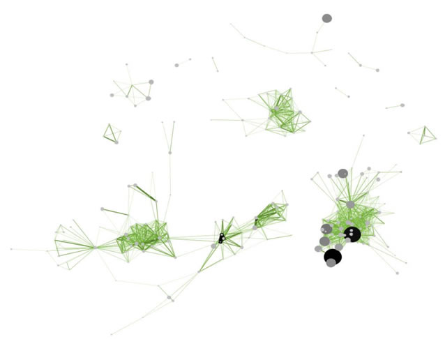
Figure 5.14: Reference co-occurrence network layout for 'FourNetSciResearchers' dataset
To see the log file from this workflow save the 5.1.4.3 Cited Reference Co-Occurrence (Bibliographic Coupling) Network log file.
5.1.4.4 Document Co-Citation Network (DCA)
Load the file using 'Load > File'' and following this path: 'yoursci2directory/sampledata/scientometrics/isi/FourNetSciResearchers.isi'. A table of all records and a table of 361 records with unique ISI ids will appear in the Data Manager.
Select the "361 Unique ISI Records" and run 'Data Preparation > Extract Paper Citation Network'. Select the 'Extracted Paper-Citation Network' and run 'Data Preparation > Extract Document Co-Citation Network.' The co-citation network will have 5,335 nodes (213 of which are isolates) and 193,039 edges. Isolates can be removed by running 'Preprocessing > Networks > Delete Isolates.' The resulting network has 5122 nodes and 193,039 edges – and is too dense for display in GUESS. Edges with low weights can be eliminated by running 'Preprocessing > Networks > Extract Edges Above or Below Value' with parameter values:
Here, only edges with a local co-citation count of five or higher are kept. The giant component in the resulting network has 265 nodes and 1,607 edges. All other components have only one or two nodes.
The giant component can be visualized in GUESS, see Figure 5.15 (right); see the above explanation, and use the same size and color coding and labeling as the bibliographic coupling network. Simply run 'GUESS: File > Run Script ...' and select 'yoursci2directory/scripts/GUESS/reference-co-occurence-nw.py'

Figure 5.15: Undirected, weighted bibliographic coupling network (left) and undirected, weighted co-citation network (right) of 'FourNetSciResearchers' dataset, with isolate nodes removed
To see the log file from this workflow save the 5.1.4.4 Document Co-Citation Network (DCA) log file.
5.1.4.5 Word Co-Occurrence Network
The Extract Word Co-Occurrence Network algorithm has been updated. To run this workflow you will need to update the plugin by downloading the edu.iu.nwb.composite.extractcowordfromtable_1.0.1.jar file and copying it into your plugins directory. Make sure to remove the old plugin: "edu.iu.nwb.composite.extractcowordfromtable_1.0.0" from the plugins directory, otherwise the new plugin will not work. If you have not updated Sci2 by adding plugins before, there are some brief directions on how to do so in 3.2 Additional Plugins.
In the Sci2 Tool, select "361 unique ISI Records" from the 'FourNetSciResearchers' dataset in the Data Manager. Run 'Preprocessing > Topical > Lowercase, Tokenize, Stem, and Stopword Text' using the following parameters:

Text normalization utilizes the Standard Analyzer provided by Lucene (http://lucene.apache.org|). It separates text into word tokens, normalizes word tokens to lower case, removes "s" from the end of words, removes dots from acronyms, deletes stop words, and applies the English Snowball stemmer (http://snowball.tartarus.org/algorithms/english/stemmer.html), which is a version of the Porter2 stemmer designed for the English language.
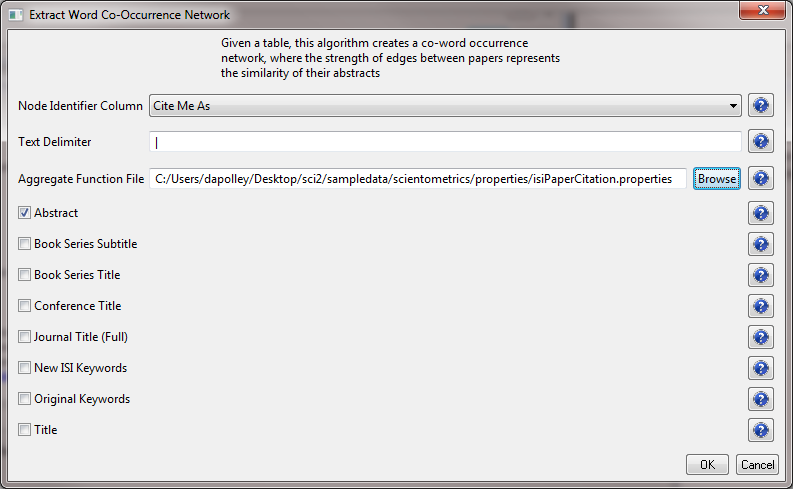
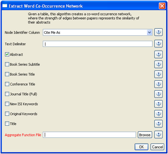
The result is a derived table – "with normalized Abstract" – in which the text in the abstract column is normalized. Select this table and run 'Data Preparation > Extract Word Co-Occurrence Network' using parameters:
Aggregate Function File
If you are working with ISI data, you can use the aggregate function file indicated in the image below. Aggregate function files can be found in sci2/sampledata/scientometrics/properties. If you are not working with ISI data and wish to create your own aggregate function file, you can find more information in 3.6 Property Files
The outcome is a network in which nodes represent words and edges and denote their joint appearance in a paper. Word co-occurrence networks are rather large and dense. Running the 'Analysis > Networks > Network Analysis Toolkit (NAT)' reveals that the network has 2,821 word nodes and 242,385 co-occurrence edges.
There are 354 isolated nodes that can be removed by running 'Preprocessing > Networks > Delete Isolates' on the Co-Word Occurrence network. Note that when isolates are removed, papers without abstracts are removed along with the keywords.
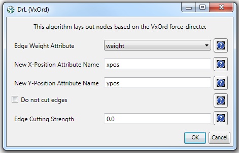
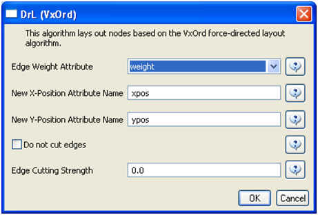
The result is one giant component with 2,467 nodes and 242,385 edges. To visualize this rather large network, begin by running 'Visualization > Networks > DrL (VxOrd)' with default values:
Note that the DrL algorithm requires extensive data processing and requires a bit of time to run, even on powerful systems. See the console window for details:

To keep only the strongest edges in the "Laid out with DrL" network, run 'Preprocessing > Networks > Extract Top Edges' on the new network using the following parameters:

Once edges have been removed, the network "top 1000 edges by weight" can be visualized by running 'Visualization > Networks > GUESS'. In GUESS, run the following commands in the Interpreter:
> for node in g.nodes:
      node.x = node.xpos * 40
      node.y = node.ypos * 40
> resizeLinear(references, 2, 40)
> colorize(references,[200,200,200],[0,0,0])
> resizeLinear(weight, .1, 2)
> g.edges.color = "127,193,65,255"
The result should look something like Figure 5.16.
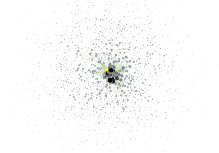
Figure 5.16: Undirected, weighted word co-occurrence network visualization for the DrL-processed 'FourNetSciResearchers' dataset
Currently, when you resize large networks in the GUESS visualization tool, the network visualizations can become "uncentered" in the display window. Running 'View > Center' does not solve this problem. Users should zoom out to find the visualization, center it, and then zoom back in.
Note that only the top 1000 edges (by weight) in this large network appear in the above visualization, creating the impression of isolate nodes. To remove nodes that are not connected by the top 1000 edges (by weight), run 'Preprocessing > Networks > Delete Isolates' on the "top 1000 edges by weight" network and visualize the result using the workflow described above.
To see the log file from this workflow save the 5.1.4.5 Word Co-Occurrence Network log file.
Database Extractions
The database plugin is not currently available for the most recent version of Sci2 (v1.0 aplpha). However, the plugin that allows files to be loaded as databases is available for Sci2 v0.5.2 alpha or older. Please check the Sci2 news page (https://sci2.cns.iu.edu/user/news.php). We will update this page when a database plugin becomes available for the latest version of the tool.
The Sci2 Tool supports the creation of databases from ISI files. Database loading improves the speed and functionality of data preparation and preprocessing. While the initial loading can take quite some time for larger datasets (see sections 3.4 Memory Allocation and 3.5 Memory Limits) it results in vastly faster and more powerful data processing and extraction.
Once again load 'yoursci2directory/sampledata/scientometrics/isi/FourNetSciResearchers.isi', this time using 'File > Load' instead of 'File > Load.' Choose 'ISI database' from the load window. Right-click to view the database schema:
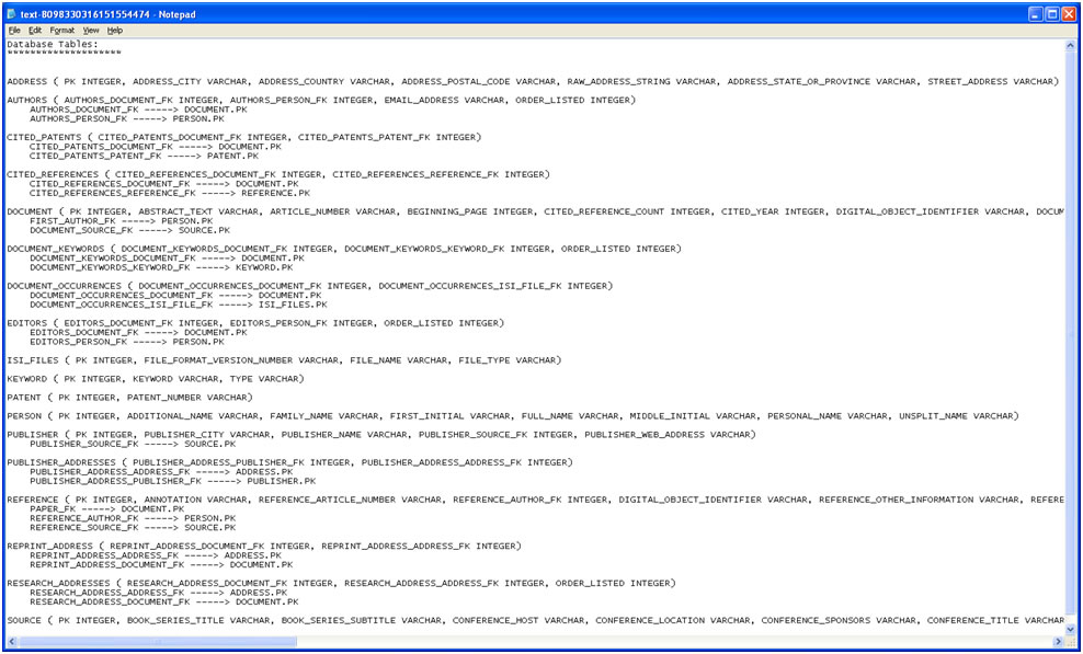
Figure 5.17: The database schema as viewed in Notepad
As before, it is important to clean the database before running any extractions by merging and matching authors, journals, and references. Run 'Data Preparation > Database > ISI > Merge Identical ISI People', followed by 'Data Preparation > Database > ISI > Merge Document Sources'' and 'Data Preparation > Database > ISI > Match References to Papers'. Make sure to wait until each cleaning step is complete before beginning the next one.
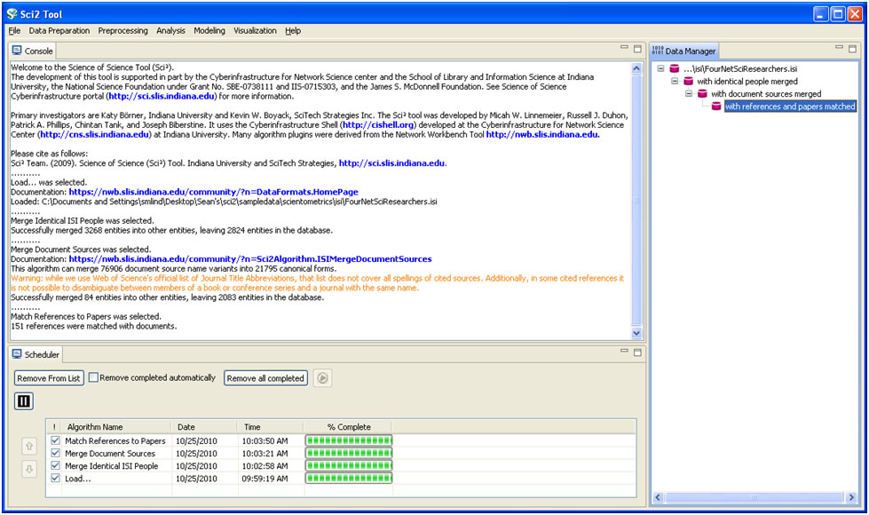
Figure 5.18: Cleaned database of 'FourNetSciResearchers'
Extracting different tables will provide different views of the data. Run 'Data Preparation > Database > ISI > Extract Authors' to view all the authors from FourNetSciResearchers.isi. The table includes the number of papers each person in the dataset authored, their Global Citation Count (how many times they have been cited according to ISI), and their Local Citation Count (how many times they were cited in the current dataset.)
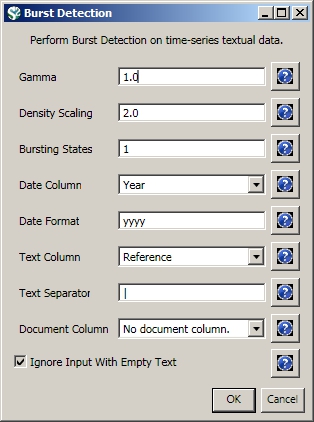
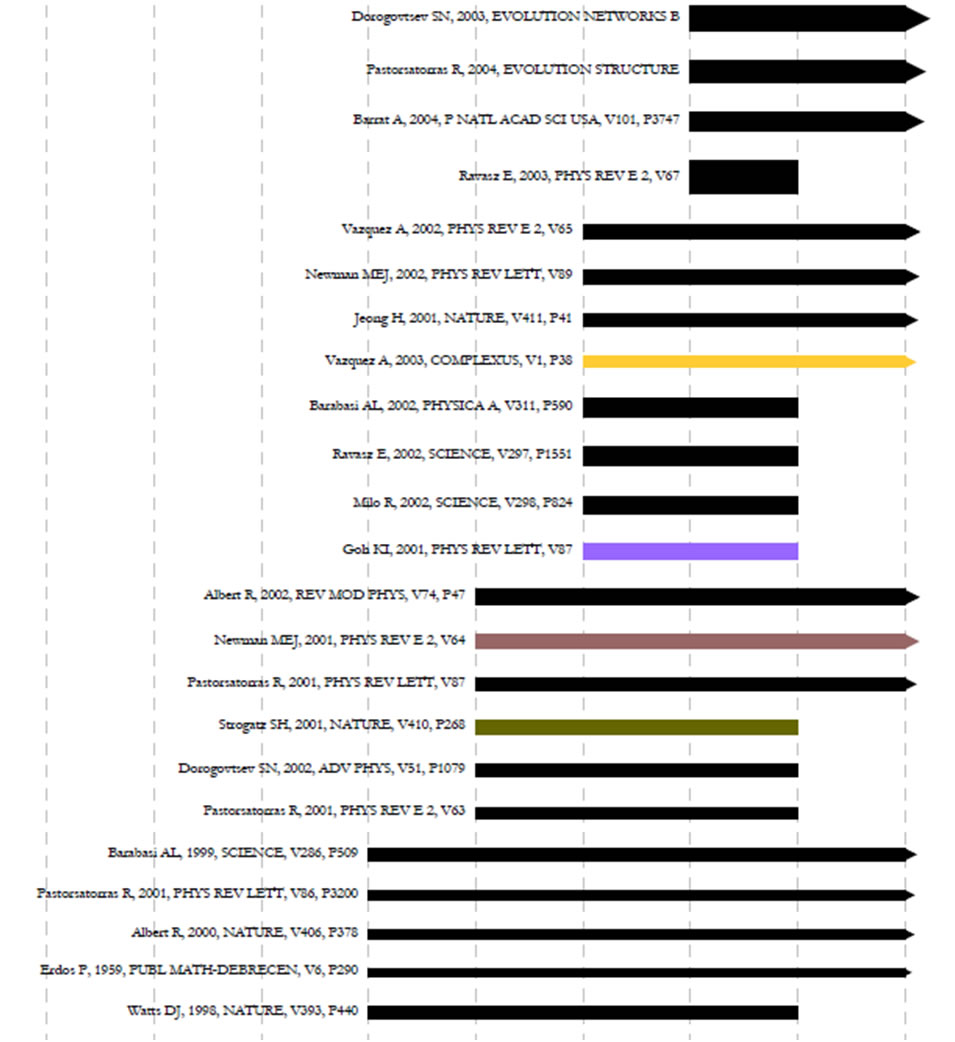
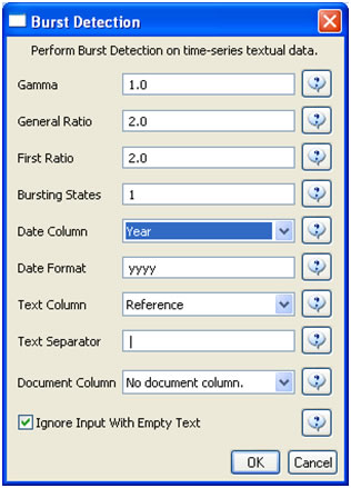
The queries can also output data specifically tailored for the burst detection algorithm (see section 4.6.1 Burst Detection).
Run 'Data Preparation > Database > ISI > Extract References by Year for Burst Detection' on the cleaned "with references and papers matched" database, followed by 'Analysis > Topical > Burst Detection' with the following parameters:
View the file "Burst detection analysis (Publication Year, Reference): maximum burst level 1". On a PC running Windows, right click on this table and select view to see the data in Excel. On a Mac or a Linux system, right click and save the file, then open using the spreadsheet program of your choice. See Burst Detection for the meaning of each field in the output.
An empty value in the "End" field indicates that the burst lasted until the last date present in the dataset. Where the "End" field is empty, manually add the last year present in the dataset. In this case, 2007.
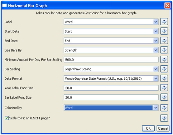
After you manually add this information, save this .csv file somewhere in your computer. Load back this .csv file into Sci2 using 'File > Load'. Select 'Standart csv format' int the pop-up window. A new table will appear in the Data Manager. To visualize this table that contains the results of the Burst Detection algorithm, select the table you just loaded in the Data Manager and run 'Visualization > Temporal > Horizontal Bar Graph' with the following parameters:
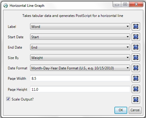
See section 2.4 Saving Visualizations for Publication to save and view the graph.
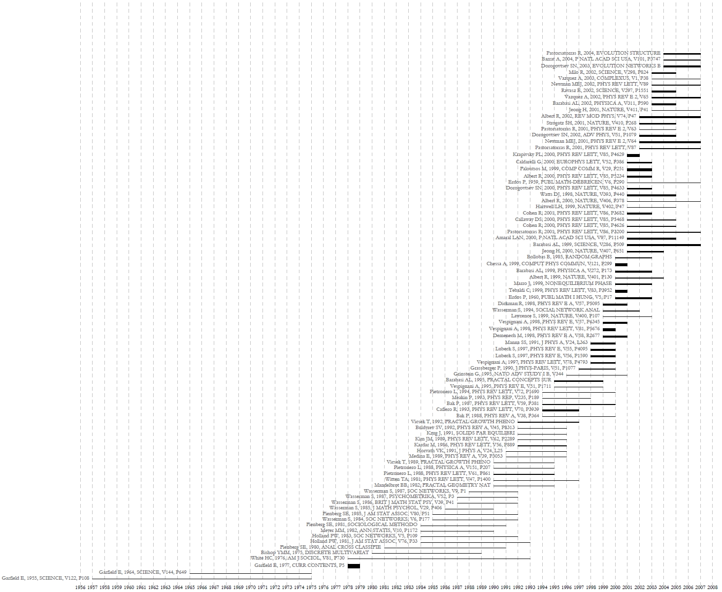
Figure 5.19: Top reference bursts in the 'FourNetSciResearchers' dataset
For temporal studies, it can be useful to aggregate data by year rather than by author, reference, etc. Running 'Data Preparation > Database > ISI > Extract Longitudinal Summary' will output a table which lists metrics for every year mentioned in the dataset. The longitudinal study table contains the volume of documents and references published per year, as well as the total number of references, the number of distinct references, distinct authors, distinct sources, and distinct keywords per year. The results are graphed in Figure 5.20 (the graph was created using Excel).
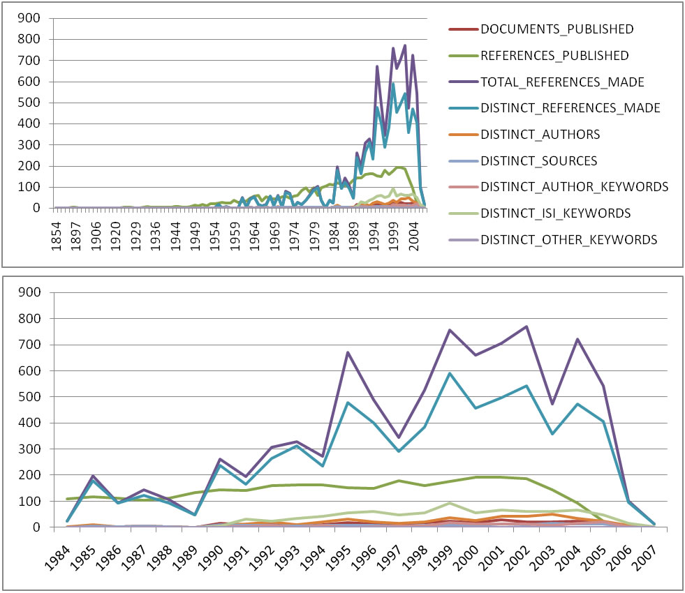
Figure 5.20: Longitudinal study of 'FourNetSciResearchers'
The largest speed increases from the database functionality can be found in the extraction of networks. First, compare the results of a co-authorship extraction with those from section 5.1.4.2 Author Co-Occurrence (Co-Author) Network. Run 'Data Preparation > Database > ISI > Extract Co-Author Network' followed by 'Analysis > Networks > Network Analysis Toolkit (NAT)'. Notice that both networks have 247 nodes and 891 edges. Visualize the extracted co-author network in GUESS using 'Visualization > Networks > GUESS' and reformat the visualization using 'Layout > GEM' and 'Layout > Bin Pack.' To apply the default co-authorship theme, go to 'Script > Run Script' and find 'yoursci2directory/scripts/GUESS/co-author-nw_database.py'. The resulting network will look like Figure 5.21.

Figure 5.21: Longitudinal study of 'FourNetSciResearchers,' visualized in GUESS
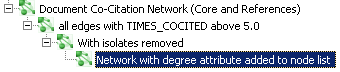
Using Sci2's database functionality allows for several network extractions that cannot be achieved with the text-based algorithms. For example, extracting journal co-citation networks reveals which journals are cited together most frequently. Run 'Data Preparation > Database > ISI > Extract Document Co-Citation Network (Core and References)' on the database to create a network of co-cited journals, and then prune it using 'Preprocessing > Networks > Extract Edges Above or Below Value' with the parameters:

Now remove isolates ('Preprocessing > Networks > Delete Isolates') and append node degree attributes to the network ('Analysis > Networks > Unweighted & Undirected > Node Degree'). The workflow in your Data Manager should look like this:
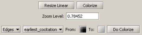
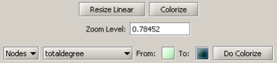
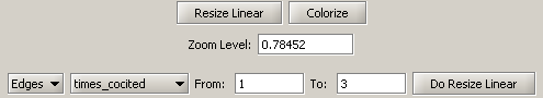
View the network in GUESS using 'Visualization > Networks > GUESS.' Use 'Layout > GEM' and 'Layout > Bin Pack' to reformat the visualization. Resize and color the edges to display the strongest and earliest co-citation links using the following parameters:


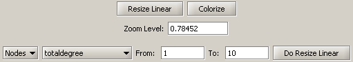
Resize, color, and label the nodes to display their degree using the following parameters:


The resulting Journal Co-Citation Analysis (JCA) appears in Figure 5.22.
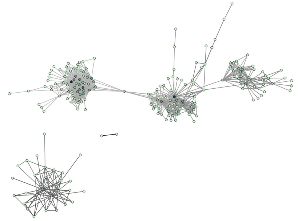
Figure 5.22: Journal co-citation analysis of 'FourNetSciResearchers,' edges with 5 or more cocitations and nodes with node degree added, visualized in GUESS